Datasets
It’s become commonplace to point out that machine learning models are only as good as the data they’re trained on. The old slogan “garbage in, garbage out” no doubt applies to machine learning practice, as does the related catchphrase “bias in, bias out”. Yet, these aphorisms still understate—and somewhat misrepresent—the significance of data for machine learning.
It’s not only the output of a learning algorithm that may suffer with poor input data. A dataset serves many other vital functions in the machine learning ecosystem. The dataset itself is an integral part of the problem formulation. It implicitly sorts out and operationalizes what the problem is that practitioners end up solving. Datasets have also shaped the course of entire scientific communities in their capacity to measure and benchmark progress, support competitions, and interface between researchers in academia and practitioners in industry.
If so much hinges on data in machine learning, it might come as a surprise that there is no simple answer to the question of what makes data good for what purpose. The collection of data for machine learning applications has not followed any established theoretical framework, certainly not one that was recognized a priori.
In this chapter, we take a closer look at popular datasets in the field of machine learning and the benchmarks that they support. We trace out the history of benchmarks and work out the implicit scientific methodology behind machine learning benchmarks. We limit the scope of this chapter in some important ways. Our focus will be largely on publicly available datasets that support training and testing purposes in machine learning research and applications. Primarily, we critically examine the train-and-test paradigm machine learning practitioners take for granted today.
The scientific basis of machine learning benchmarks
Methodologically, much of modern machine learning practice rests on a variant of trial and error, which we call the train-test paradigm. Practitioners repeatedly build models using any number of heuristics and test their performance to see what works. Anything goes as far as training is concerned, subject only to computational constraints, so long as the performance looks good in testing. Trial and error is sound so long as the testing protocol is robust enough to absorb the pressure placed on it. We will examine to which extent this is the case in machine learning.
From a theoretical perspective, the best way to test the performance of a predictor f is to collect a sufficiently large fresh dataset S and to compute the empirical risk R_S[f]. We already learned that the empirical risk in this case is an unbiased estimate of the risk of the predictor. For a bounded loss function and a test set of size n, an appeal to Hoeffding’s inequality proves the generalization gap to be no worse than O(1/\sqrt{n}). We can go a step further and observe that if we take union bound over k fixed predictors, our fresh sample will simultaneously provide good estimates for all k predictors up to a maximum error of O(\sqrt{\log(k)/n}). In fact, we can apply any of the mathematical tools we saw in the Generalization chapter so long as the sample S really is a fresh sample with respect to the set of models we want to evaluate.
Data collection, however, is a difficult and costly task. In most applications, practitioners cannot sample fresh data for each model they would like to try out. A different practice has therefore become the de facto standard. Practitioners split their dataset into typically two parts, a training set used for training a model, and a test set used for evaluating its performance. Sometimes practitioners divide their data into multiple splits, e.g., training, validation, and test sets. However, for our discussion here that won’t be necessary. Often the split is determined when the dataset is created. Datasets used for benchmarks in particular have one fixed split persistent throughout time. A number of variations on this theme go under the name holdout method.
Machine learning competitions have adopted the same format. The company Kaggle, for example, has organized hundreds of competitions since it was founded. In a competition, a holdout set is kept secret and is used to rank participants on a public leaderboard as the competition unfolds. In the end, the final winner is whoever scores highest on a separate secret test set not used to that point.
In all applications of the holdout method the hope is that the test set will serve as a fresh sample that provides good risk estimates for all the models. The central problem is that practitioners don’t just use the test data once only to retire it immediately thereafter. The test data are used incrementally for building one model at a time while incorporating feedback received previously from the test data. This leads to the fear that eventually models begin to overfit to the test data.
Duda and Hart summarize the problem aptly in their 1973 textbook:
In the early work on pattern recognition, when experiments were often done with very small numbers of samples, the same data were often used for designing and testing the classifier. This mistake is frequently referred to as “testing on the training data.” A related but less obvious problem arises when a classifier undergoes a long series of refinements guided by the results of repeated testing on the same data. This form of “training on the testing data” often escapes attention until new test samples are obtained.Duda and Hart, Pattern Classification and Scene Analysis (Wiley New York, 1973).
Nearly half a century later, Hastie, Tibshirani, and Friedman still caution in the 2017 edition of their influential textbook:
Ideally, the test set should be kept in a “vault,” and be brought out only at the end of the data analysis. Suppose instead that we use the test-set repeatedly, choosing the model with smallest test-set error. Then the test set error of the final chosen model will underestimate the true test error, sometimes substantially.Hastie, Tibshirani, and Friedman, The Elements of Statistical Learning: Data Mining, Inference, and Prediction (Corrected 12th Printing) (Springer, 2017).
Indeed, reuse of test data—on the face of it—invalidates the statistical guarantees of the holdout method. The predictors created with knowledge about prior test-set evaluations are no longer independent of the test data. In other words, the sample isn’t fresh anymore. While the suggestion to keep the test data in a “vault” is safe, it couldn’t be further from the reality of modern practice. Popular test datasets often see tens of thousands of evaluations.
We could try to salvage the situation by relying on uniform convergence. If all models we try out have sufficiently small complexity in some formal sense, such as VC-dimension, we could use the tools from the Generalization chapter to negotiate some sort of a bound. However, the whole point of the train-test paradigm is not to constrain the complexity of the models a priori, but rather to let the practitioner experiment freely. Moreover, if we had an actionable theoretical generalization guarantee to begin with, there would hardly be any need for the holdout method whose purpose is to provide an empirical estimate where theoretical guarantees are lacking.
Before we discuss the “training on the testing data” problem any further, it’s helpful to get a better sense of concrete machine learning benchmarks, their histories, and their impact within the community.
A tour of datasets in different domains
The creation of datasets in machine learning does not follow a clear theoretical framework. Datasets aren’t collected to test a specific scientific hypothesis. In fact, we will see that there are many different roles data plays in machine learning. As a result, it makes sense to start by looking at a few influential datasets from different domains to get a better feeling for what they are, what motivated their creation, how they organized communities, and what impact they had.
TIMIT
Automatic speech recognition is a machine learning problem of significant commercial interest. Its roots date back to the early 20th century.Li and Mills, “Vocal Features: From Voice Identification to Speech Recognition by Machine,” Technology and Culture 60, no. 2 (2019): S129–60.
Interestingly, speech recognition also features one of the oldest benchmarks datasets, the TIMIT (Texas Instruments/Massachusetts Institute for Technology) data. The creation of the dataset was funded through a 1986 DARPA program on speech recognition. In the mid-eighties, artificial intelligence was in the middle of a “funding winter” where many governmental and industrial agencies were hesitant to sponsor AI research because it often promised more than it could deliver. DARPA program manager Charles Wayne proposed a way around this problem was establishing more rigorous evaluation methods. Wayne enlisted the National Institute of Standards and Technology to create and curate shared datasets for speech, and he graded success in his program based on performance on recognition tasks on these datasets.
Many now credit Wayne’s program with kick starting a revolution of progress in speech recognition.Liberman, “Obituary: Fred Jelinek,” Computational Linguistics 36, no. 4 (2010): 595–99; Church, “Emerging Trends: A Tribute to Charles Wayne,” Natural Language Engineering 24, no. 1 (2018): 155–60; Liberman and Wayne, “Human Language Technology,” AI Magazine 41, no. 2 (2020): 22–35. According to Church,
It enabled funding to start because the project was glamour-and-deceit-proof, and to continue because funders could measure progress over time. Wayne’s idea makes it easy to produce plots which help sell the research program to potential sponsors. A less obvious benefit of Wayne’s idea is that it enabled hill climbing. Researchers who had initially objected to being tested twice a year began to evaluate themselves every hour.Church, “Emerging Trends.”
A first prototype of the TIMIT dataset was released in December of 1988 on a CD-ROM. An improved release followed in October 1990. TIMIT already featured the training/test split typical for modern machine learning benchmarks. There’s a fair bit we know about the creation of the data due to its thorough documentation.Garofolo et al., “DARPA TIMIT Acoustic-Phonetic Continuous Speech Corpus CD-ROM. NIST Speech Disc 1-1.1,” STIN 93 (1993): 27403.
TIMIT features a total of about 5 hours of speech, composed of 6300 utterances, specifically, 10 sentences spoken by each of 630 speakers. The sentences were drawn from a corpus of 2342 sentences such as the following.
She had your dark suit in greasy wash water all year. (sa1)
Don't ask me to carry an oily rag like that. (sa2)
This was easy for us. (sx3)
Jane may earn more money by working hard. (sx4)
She is thinner than I am. (sx5)
Bright sunshine shimmers on the ocean. (sx6)
Nothing is as offensive as innocence. (sx7)
The TIMIT documentation distinguishes between 8 major dialect regions in the United States:
New England, Northern, North Midland, South Midland, Southern, New York City, Western, Army Brat (moved around)
Of the speakers, 70% are male and 30% are female. All native speakers of American English, the subjects were primarily employees of Texas Instruments at the time. Many of them were new to the Dallas area where they worked.
Racial information was supplied with the distribution of the data and coded as “White”, “Black”, “American Indian”, “Spanish-American”, “Oriental”, and “Unknown”. Of the 630 speakers, 578 were identified as White, 26 as Black, 2 as American Indian, 2 as Spanish-American, 3 as Oriental, and 17 as unknown.
| Male | Female | Total (%) | |
|---|---|---|---|
| White | 402 | 176 | 578 (91.7%) |
| Black | 15 | 11 | 26 (4.1%) |
| American Indian | 2 | 0 | 2 (0.3%) |
| Spanish-American | 2 | 0 | 2 (0.3%) |
| Oriental | 3 | 0 | 3 (0.5%) |
| Unknown | 12 | 5 | 17 (2.6%) |
The documentation notes:
In addition to these 630 speakers, a small number of speakers with foreign accents or other extreme speech and/or hearing abnormalities were recorded as “auxiliary” subjects, but they are not included on the CD-ROM.
It comes to no surprise that early speech recognition models had significant demographic and racial biases in their performance.
Today, several major companies, including Amazon, Apple, Google, and Microsoft, all use speech recognition models in a variety of products from cell phone apps to voice assistants. Today, speech recognition lacks a major open benchmark that would support the training models competitive with the industrial counterparts. Industrial speech recognition pipelines are often complex systems that use proprietary data sources that not a lot is known about. Nevertheless, even today’s speech recognition systems continue to have racial biases.Koenecke et al., “Racial Disparities in Automated Speech Recognition,” Proceedings of the National Academy of Sciences 117, no. 14 (2020): 7684–89.
UCI Machine Learning Repository
The UCI Machine Learning Repository currently hosts more than 500 datasets, mostly for different classification and regression tasks. Most datasets are relatively small, many of them structured tabular datasets with few attributes.
The UCI Machine Learning Repository contributed to the adoption of the train-test paradigm in machine learning in the late 1980s. Langley recalls:
The experimental movement was aided by another development. David Aha, then a PhD student at UCI, began to collect datasets for use in empirical studies of machine learning. This grew into the UCI Machine Learning Repository (), which he made available to the community by FTP in 1987. This was rapidly adopted by many researchers because it was easy to use and because it let them compare their results to previous findings on the same tasks.Langley, “The Changing Science of Machine Learning” (Springer, 2011).
Aha’s PhD work involved evaluating nearest-neighbor methods, and he wanted to be able to compare the utility of his algorithms to decision tree induction algorithms, popularized by Ross Quinlan. Aha describes his motivation for building the UCI repository as follows.
I was determined to create and share it, both because I wanted to use the datasets for my own research and because I thought it was ridiculous that the community hadn’t fielded what should have been a useful service. I chose to use the simple attribute-value representation that Ross Quinlan was using so successfully for distribution with his TDIDT implementations.Aha (Personal communication, 2020).
The UCI dataset was wildly successful, and partially responsible for the renewed interest in pattern recognition methods in machine learning. However, this success came with some detractors. By the mid 1990s, many were worried that evaluation-by-benchmark encouraged chasing state-of-the-art results and writing incremental papers. Aha reflects:
By ICML-95, the problems “caused” by the repository had become popularly espoused. For example, at that conference Lorenza Saitta had, in an invited workshop that I co-organized, passionately decried how it allowed researchers to publish dull papers that proposed small variations of existing supervised learning algorithms and reported their small-but-significant incremental performance improvements in comparison studies.
Nonetheless, the UCI repository remains one of the most popular source for benchmark datasets in machine learning, and many of the early datasets still are used for benchmarking in machine learning research. The most popular dataset in the UCI repository is Ronald A. Fisher’s Iris Data Set that Fisher collected for his 1936 paper on “The use of multiple measurements in taxonomic problems”.
As of writing, the second most popular dataset in the UCI repository is the Adult dataset. Extracted from the 1994 Census database, the dataset features nearly 50,000 instances describing individual in the United States, each having 14 attributes. The goal is to classify whether an individual earns more than 50,000 US dollars or less.
The Adult dataset became popular in the algorithmic fairness community, largely because it is one of the few publicly available datasets that features demographic information including gender (coded in binary as male/female), as well as race (coded as Amer-Indian-Eskimo, Asian-Pac-Islander, Black, Other, and White).
Unfortunately, the data has some idiosyncrasies that make it less than ideal for understanding biases in machine learning models.Ding et al., “Retiring Adult: New Datasets for Fair Machine Learning,” in Advances in Neural Information Processing Systems, 2021. Due to the age of the data, and the income cutoff at $50,000, almost all instances labeled Black are below the cutoff, as are almost all instances labeled female. Indeed, a standard logistic regression model trained on the data achieves about 85% accuracy overall, while the same model achieves 91% accuracy on Black instances, and nearly 93% accuracy on female instances. Likewise, the ROC curves for the latter two groups enclose actually more area than the ROC curve for male instances. This is a rather untypical situation since often machine learning models perform more poorly on historically disadvantaged groups.
Highleyman’s data
The first machine learning benchmark dates back to the late 1950s. Few used it and even fewer still remembered it by the time benchmarks became widely used in machine learning in the late 1980s.
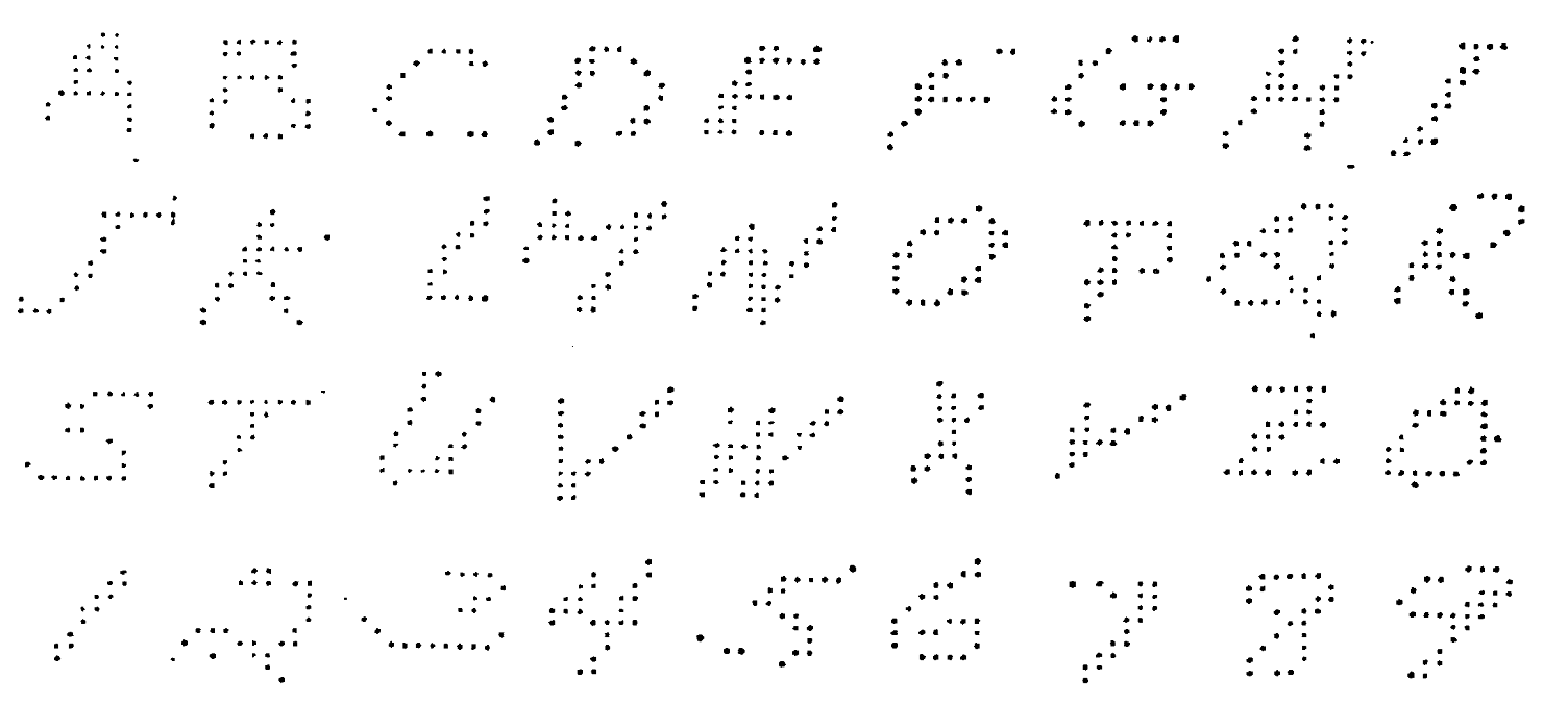
In 1959 at Bell Labs, Bill Highleyman and Louis Kamenstky designed a scanner to evaluate character recognition techniques.Highleyman and Kamentsky, “A Generalized Scanner for Pattern- and Character-Recognition Studies,” in Western Joint Computer Conference, 1959, 291–94. Their goal was “to facilitate a systematic study of character-recognition techniques and an evaluation of methods prior to actual machine development.” It was not clear at the time which part of the computations should be done in special purpose hardware and which parts should be done with more general computers. Highleyman later patented an optical character recognition (OCR) scheme that we recognize today as a convolutional neural network with convolutions optically computed as part of the scanning.Highleyman, “Character Recognition System” (Google Patents, 1961).
Highleyman and Kamentsky used their scanner to create a data set of 1800 alphanumeric characters. They gathered the 26 capital letters of the English alphabet and 10 digits from 50 different writers. Each character in their corpus was scanned in binary at a resolution of 12 x 12 and stored on punch cards that were compatible with the IBM 704, the first mass-produced computer with floating-point arithmetic hardware.
With the data in hand, Highleyman and Kamenstky began studying various proposed techniques for recognition. In particular, they analyzed a method of Woody Bledsoe’s and published an analysis claiming to be unable to reproduce the results.Highleyman and Kamentsky, “Comments on a Character Recognition Method of Bledsoe and Browning,” IRE Transactions on Electronic Computers EC–9, no. 2 (1960): 263–63. Bledsoe found the numbers to be considerably lower than he expected, and asked Highleyman to send him the data. Highleyman obliged, mailing the package of punch cards across the country to Sandia Labs. Upon receiving the data, Bledsoe conducted a new experiment. In what may be the first application of the train-test split, he divided the characters up, using 40 writers for training and 10 for testing. By tuning the hyperparameters, Bledsoe was able to achieve approximately 60% error.Bledsoe, “Further Results on the n-Tuple Pattern Recognition Method,” IRE Transactions on Electronic Computers EC–10, no. 1 (1961): 96–96. Bledsoe also suggested that the high error rates were to be expected as Highleyman’s data was too small. Prophetically, he declared that 1000 alphabets might be needed for good performance.
By this point, Highleyman had also shared his data with Chao Kong Chow at the Burroughs Corporation (a precursor to Unisys). A pioneer of using decision theory for pattern recognition,Chow, “An Optimum Character Recognition System Using Decision Functions,” IRE Transactions on Electronic Computers, no. 4 (1957): 247–54. Chow built a pattern recognition system for characters. Using the same train-test split as Bledsoe, Chow obtained an error rate of 41.7%.Chow, “A Recognition Method Using Neighbor Dependence,” IRE Transactions on Electronic Computers EC–11, no. 5 (1962): 683–90.
Highleyman made at least six additional copies of the data he had sent to Bledsoe and Chow, and many researchers remained interested. He thus decided to publicly offer to send a copy to anyone willing to pay for the duplication and shipping fees.Highleyman, “Data for Character Recognition Studies,” IEEE Transactions on Electronic Computers EC–12, no. 2 (1963): 135–36. Of course, the dataset was sent by US Postal Service. Electronic transfer didn’t exist at the time, resulting in sluggish data transfer rates on the order of a few bits per minute.
Highleyman not only created the first machine learning benchmark. He authored the first formal study of train-test splitsHighleyman, “The Design and Analysis of Pattern Recognition Experiments,” The Bell System Technical Journal 41, no. 2 (1962): 723–44. and proposed empirical risk minimization for pattern classificationHighleyman, “Linear Decision Functions, with Application to Pattern Recognition,” Proceedings of the IRE 50, no. 6 (1962): 1501–14. as part of his 1961 dissertation. By 1963, however, Highleyman had left his research position at Bell Labs and abandoned pattern recognition research.
We don’t know how many people requested Highleyman’s data, but the total number of copies may have been less than twenty. Based on citation surveys, we determined there were at least six additional copies made after Highleyman’s public offer for duplication, sent to researchers at UW Madison, CMU, Honeywell, SUNY Stony Brook, Imperial College in London, and Stanford Research Institute (SRI).
The SRI team of John Munson, Richard Duda, and Peter Hart performed some of the most extensive experiments with Highleyman’s data.Munson, Duda, and Hart, “Experiments with Highleyman’s Data,” IEEE Transactions on Computers C–17, no. 4 (1968): 399–401. A 1-nearest-neighbors baseline achieved an error rate of 47.5%. With a more sophisticated approach, they were able to do significantly better. They used a multi-class, piecewise linear model, trained using Kesler’s multi-class version of the perceptron algorithm. Their feature vectors were 84 simple pooled edge detectors in different regions of the image at different orientations. With these features, they were able to get a test error of 31.7%, 10 points better than Chow. When restricted only to digits, this method recorded 12% error. The authors concluded that they needed more data, and that the error rates were “still far too high to be practical.” They concluded that “larger and higher-quality datasets are needed for work aimed at achieving useful results.” They suggested that such datasets “may contain hundreds, or even thousands, of samples in each class.”
Munson, Duda, and Hart also performed informal experiments with humans to gauge the readability of Highleyman’s characters. On the full set of alphanumeric characters, they found an average error rate of 15.7%, about 2x better than their pattern recognition machine. But this rate was still quite high and suggested the data needed to be of higher quality. They concluded that “an array size of at least 20X20 is needed, with an optimum size of perhaps 30X30.”
Decades passed until such a dataset, the MNIST digit recognition task, was created and made widely available.
MNIST
The MNIST dataset contains images of handwritten digits. Its most common version has 60,000 training images and 10,000 test images, each having 28x28 grayscale pixels.
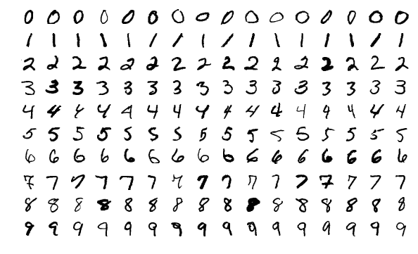
MNIST was created by researchers Burges, Cortes, and LeCun from data by the National Institute of Standards and Technology (NIST). The dataset was introduced in a research paper in 1998 to showcase the use of gradient-based deep learning methods for document recognition tasks.LeCun et al., “Gradient-Based Learning Applied to Document Recognition,” Proceedings of the IEEE 86, no. 11 (1998): 2278–2324. However, the authors released the dataset to provide a convenient benchmark of image data, in contrast to UCI’s predominantly tabular data. The MNIST website states
It is a good database for people who want to try learning techniques and pattern recognition methods on real-world data while spending minimal efforts on preprocessing and formatting.LeCun (http://yann.lecun.com/exdb/mnist/, n.d.).
MNIST became a highly influential benchmark in the machine learning community. Two decades and over 30,000 citation later, researchers continue to use the data actively.
The original NIST data had the property that training and test data came from two different populations. The former featured the handwriting of two thousand American Census Bureau employees, whereas the latter came from five hundred American high school students.Grother, “NIST Special Database 19 Handprinted Forms and Characters Database,” National Institute of Standards and Technology, 1995. The creators of MNIST reshuffled these two data sources and split them into training and test set. Moreover, they scaled and centered the digits. The exact procedure to derive MNIST from NIST was lost, but recently reconstructed by matching images from both data sources.Yadav and Bottou, “Cold Case: The Lost MNIST Digits,” in Advances in Neural Information Processing Systems, 2019, 13443–52.
The original MNIST test set was of the same size as the training set, but the smaller test set became standard in research use. The 50,000 digits in the original test set that didn’t make it into the smaller test set were later identified and dubbed the lost digits.Yadav and Bottou.
From the beginning, MNIST was intended to be a benchmark used to compare the strengths of different methods. For several years, LeCun maintained an informal leaderboard on a personal website that listed the best accuracy numbers that different learning algorithms achieved on MNIST.
| Method | Test error (%) |
|---|---|
| linear classifier (1-layer NN) | 12.0 |
| linear classifier (1-layer NN) [deskewing] | 8.4 |
| pairwise linear classifier | 7.6 |
| K-nearest-neighbors, Euclidean | 5.0 |
| K-nearest-neighbors, Euclidean, deskewed | 2.4 |
| 40 PCA + quadratic classifier | 3.3 |
| 1000 RBF + linear classifier | 3.6 |
| K-NN, Tangent Distance, 16x16 | 1.1 |
| SVM deg 4 polynomial | 1.1 |
| Reduced Set SVM deg 5 polynomial | 1.0 |
| Virtual SVM deg 9 poly [distortions] | 0.8 |
| 2-layer NN, 300 hidden units | 4.7 |
| 2-layer NN, 300 HU, [distortions] | 3.6 |
| 2-layer NN, 300 HU, [deskewing] | 1.6 |
| 2-layer NN, 1000 hidden units | 4.5 |
| 2-layer NN, 1000 HU, [distortions] | 3.8 |
| 3-layer NN, 300+100 hidden units | 3.05 |
| 3-layer NN, 300+100 HU [distortions] | 2.5 |
| 3-layer NN, 500+150 hidden units | 2.95 |
| 3-layer NN, 500+150 HU [distortions] | 2.45 |
| LeNet-1 [with 16x16 input] | 1.7 |
| LeNet-4 | 1.1 |
| LeNet-4 with K-NN instead of last layer | 1.1 |
| LeNet-4 with local learning instead of ll | 1.1 |
| LeNet-5, [no distortions] | 0.95 |
| LeNet-5, [huge distortions] | 0.85 |
| LeNet-5, [distortions] | 0.8 |
| Boosted LeNet-4, [distortions] | 0.7 |
In its capacity as a benchmark, it became a showcase for the emerging kernel methods of the early 2000s that temporarily achieved top performance on MNIST.Decoste and Schölkopf, “Training Invariant Support Vector Machines,” Machine Learning 46, no. 1–3 (2002): 161–90. Today, it is not difficult to achieve less than 0.5% classification error with a wide range of convolutional neural network architectures. The best models classify all but a few pathological test instances correctly. As a result, MNIST is widely considered too easy for today’s research tasks.
MNIST wasn’t the first dataset of handwritten digits in use for machine learning research. Earlier, the US Postal Service (USPS) had released a dataset of 9298 images (7291 for training, and 2007 for testing). The USPS data was actually a fair bit harder to classify than MNIST. A non-negligible fraction of the USPS digits look unrecognizable to humans,Bromley and Sackinger, “Neural-Network and k-Nearest-Neighbor Classifiers,” Rapport Technique, 1991, 11359–910819. whereas humans recognize essentially all digits in MNIST.
ImageNet
ImageNet is a large repository of labeled images that has been highly influential in computer vision research over the last decade. The image labels correspond to nouns from the WordNet lexical database of the English language. WordNet groups nouns into cognitive synonyms, called synsets. The words car and automobile, for example, would fall into the same synset. On top of these categories, WordNet provides a hierarchical structure according to a super-subordinate relationship between synsets. The synset for chair, for example, is a child of the synset for furniture in the wordnet hierarchy. WordNet existed before ImageNet and in part inspired the creation of ImageNet.
The initial release of ImageNet included about 5000 image categories each corresponding to a synset in WordNet. These ImageNet categories averaged about 600 images per category.Deng et al., “ImageNet: A Large-Scale Hierarchical Image Database,” in Computer Vision and Pattern Recognition, 2009, 248–55. ImageNet grew over time and its Fall 2011 release had reached about 32,000 categories.
The construction of ImageNet required two essential steps:
- The first was the retrieval of candidate images for each synset.
- The second step in the creation process was the labeling of images.
Scale was an important consideration due to the target size of the image repository.
This first step utilized available image databases with a search interface, specifically, Flickr. Candidate images were taken from the image search results associated with the synset nouns for each category.
For the second labeling step, the creators of ImageNet turned to Amazon’s Mechanical Turk platform (MTurk). MTurk is an online labor market that allows individuals and corporations to hire on-demand workers to perform simple tasks. In this case, MTurk workers were presented with candidate images and had to decide whether or not the candidate image was indeed an image corresponding to the category that it was putatively associated with.
It is important to distinguish between this ImageNet database and a popular machine learning benchmark and competition, called ImageNet Large Scale Visual Recognition Challenge (ILSVRC), that was derived from it.Russakovsky et al., “ImageNet Large Scale Visual Recognition Challenge,” International Journal of Computer Vision 115, no. 3 (2015): 211–52. The competition was organized yearly from 2010 until 2017 to “measure the progress of computer vision for large scale image indexing for retrieval and annotation.” In 2012, ILSVRC reached significant notoriety in both industry and academia when a deep neural network trained by Krizhevsky, Sutskever, and Hinton outperformed all other models by a significant margin.Krizhevsky, Sutskever, and Hinton, “ImageNet Classification with Deep Convolutional Neural Networks,” in Advances in Neural Information Processing Systems, 2012. This result—yet again an evaluation in a train-test paradigm—helped usher in the latest era of exuberant interest in machine learning and neural network models under the rebranding as deep learning.Malik, “What Led Computer Vision to Deep Learning?” Communications of the ACM 60, no. 6 (2017): 82–83.
When machine learning practitioners say “ImageNet” they typically refer to the data used for the image classification task in the 2012 ILSVRC benchmark. The competition included other tasks, such as object recognition, but image classification has become the most popular task for the dataset. Expressions such as “a model trained on ImageNet” typically refer to training an image classification model on the benchmark dataset from 2012.
Another common practice involving the ILSVRC data is pre-training. Often a practitioner has a specific classification problem in mind whose label set differs from the 1000 classes present in the data. It’s possible nonetheless to use the data to create useful features that can then be used in the target classification problem. Where ILSVRC enters real-world applications it’s often to support pre-training.
This colloquial use of the word ImageNet can lead to some confusion, not least because the ILSVRC-2012 dataset differs significantly from the broader database. It only includes a subset of 1000 categories. Moreover, these categories are a rather skewed subset of the broader ImageNet hierarchy. For example, of these 1000 categories only three are in the person branch of the WordNet hierarchy, specifically, groom, baseball player, and scuba diver. Yet, more than 100 of the 1000 categories correspond to different dog breeds. The number is 118, to be exact, not counting wolves, foxes, and wild dogs that are also present among the 1000 categories.
What motivated the exact choice of these 1000 categories is not entirely clear. The apparent canine inclination, however, isn’t just a quirk either. At the time, there was an interest in the computer vision community in making progress on prediction with many classes, some of which are very similar. This reflects a broader pattern in the machine learning community. The creation of datasets is often driven by an intuitive sense of what the technical challenges are for the field. In the case of ImageNet, scale, both in terms of the number of data points as well as the number of classes, was an important motivation.
The large scale annotation and labeling of datasets, such as we saw in the case of ImageNet, fall into a category of labor that anthropologist Gray and computer scientist Suri coined Ghost Work in their book of the same name.Gray and Suri, Ghost Work: How to Stop Silicon Valley from Building a New Global Underclass (Eamon Dolan Books, 2019). They point out:
MTurk workers are the AI revolution’s unsung heroes.
Indeed, ImageNet was labeled by about 49,000 MTurk workers from 167 countries over the course of multiple years.
Longevity of benchmarks
The holdout method is central to the scientific and industrial activities of the machine learning community. Thousands of research papers have been written that report numbers on popular benchmark data, such as MNIST, CIFAR-10, or ImageNet. Often extensive tuning and hyperparameter optimization went into each such research project to arrive at the final accuracy numbers reported in the paper.
Does this extensive reuse of test sets not amount to what Duda and Hart call the “training on the testing data” problem? If so, how much of the progress that has been made is real, and how much amounts of overfitting to the test data?
To answer these questions we will develop some more theory that will help us interpret the outcome of empirical meta studies into the longevity of machine learning benchmarks.
The problem of adaptivity
Model building is an iterative process where the performance of a model informs subsequent design choices. This iterative process creates a closed feedback loop between the practitioner and the test set. In particular, the models the practitioner chooses are not independent of the test set, but rather adaptive.
Adaptivity can be interpreted as a form of overparameterization. In an adaptively chosen sequence of predictors f_1,\dots,f_k, the k-th predictor had the ability to incorporate at least k-1 bits of information about the performance of previously chosen predictors. This suggests that as k\ge n, the statistical guarantees of the holdout method become vacuous. This intuition is formally correct, as we will see.
To reason about adaptivity, it is helpful to frame the problem as an interaction between two parties. One party holds the dataset S. Think of this party as implementing the holdout method. The other party, we call analyst, can query the dataset by requesting the empirical risk R_S[f] of a given predictor f on the dataset S. The parties interact for some number k of rounds, thus creating a sequence of adaptively chosen predictors f_1,\dots,f_k. Keep in mind that this sequence depends on the dataset! In particular, when S is drawn at random, f_2,\dots, f_k become random variables, too, that are in general not independent of each other.

In general, the estimate R_t returned by the holdout mechanism at step t need not be equal to R_S[f_t]. We can often do better than the standard holdout mechanism by limiting the information revealed by each response. Throughout this chapter, we restrict our attention to the case of the zero-one loss and binary prediction, although the theory extends to other settings.
As it turns out, the guarantee of the standard holdout mechanism in the adaptive case is exponentially worse in k compared with the non-adaptive case. Indeed, there is a fairly natural sequence of k adaptively chosen predictors, resembling the practice of ensembling, on which the empirical risk is off by at least \Omega(\sqrt{k/n}). This is a lower bound on the gap between risk and empirical risk in the adaptive setting. Contrast this with the O(\sqrt{\log(k)/n}) upper bound that we observed for the standard holdout mechanism in the non-adaptive case. We present the idea for the zero-one loss in a binary prediction problem.
Overfitting by ensembling:
- Choose k of random binary predictors f_1,\dots, f_k.
- Compute the set I=\{i\in[k]\colon R_S[f_i] < 1/2\}.
- Output the predictor f=\mathrm{majority}\{ f_i \colon i\in I \} that takes a majority vote over all the predictors computed in the second step.
The key idea of the algorithm is to select all the predictors that have accuracy strictly better than random guessing. This selection step creates a bias that gives each selected predictor an advantage over random guessing. The majority vote in the third step amplifies this initial advantage into a larger advantage that grows with k. The next proposition confirms that indeed this strategy finds a predictor whose empirical risk is bounded away from 1/2 (random guessing) by a margin of \Omega(\sqrt{k/n}). Since the predictor does nothing but taking a majority vote over random functions, its risk is of course no better than 1/2.
For sufficiently large k\le n, overfitting by ensembling returns a predictor f whose classification error satisfies with probability 1/3, R_S[f]\le \frac12-\Omega(\sqrt{k/n})\,. In particular, \Delta_{\mathrm{gen}}(f)\ge\Omega(\sqrt{k/n}).
We also have a nearly matching upper bound that essentially follows from a Hoeffding’s concentration inequality just as the cardinality bound in the previous chapter. However, in order to apply Hoeffding’s inequality we first need to understand a useful idea about how we can analyze the adaptive setting.
The idea is that we can think of the interaction between a fixed analyst \mathcal{A} and the dataset as a tree. The root node is labeled by f_1=\mathcal{A}(\emptyset), i.e., the first function that the analyst queries without any input. The response R_S[f_1] takes on n+1 possible values. This is because we consider the zero-one loss, which can only take the values \{0, 1/n, 2/n,\dots, 1\}. Each possible response value a_1 creates a new child node in the tree corresponding to the function f_2=\mathcal{A}(a_1) that the analyst queries upon receiving answer a_1 to the first query f_1. We recursively continue the process until we built up a tree of depth k and degree n+1 at each node.

Note that this tree only depends on the analyst and how it responds to possible query answers, but it does not depend on the actual query answers we get out of the sample S. The tree is therefore data-independent. This argument is useful in proving the following proposition.
For any sequence of k adaptively chosen predictors f_1,\dots, f_k, the holdout method satisfies with probability 2/3, \max_{1\le t\le k} \Delta_{\mathrm{gen}}(f_t) \le O\left(\sqrt{k\log(n+1)/n}\right)\,.
The adaptive analyst defines a tree of depth k and degree n+1. Let F be the set of functions appearing at any of the nodes in the tree. Note that |F|\le (n+1)^k.
Since this set of functions is data independent, we can apply the cardinality bound from the previous chapter to argue that the maximum generalization gap for any function in F is bounded by O(\sqrt{\log|F|/n}) with any constant probability. But the functions f_1,\dots, f_k are contained in F by construction. Hence, the claim follows.
These propositions show that the principal concern of “training on the testing data” is not unfounded. In the worst case, holdout data can lose its guarantees rather quickly. If this pessimistic bound manifested in practice, popular benchmark datasets would quickly become useless. But does it?
Replication efforts
In recent replication efforts, researchers carefully recreated new test sets for the CIFAR-10 and ImageNet classification benchmarks, created according to the very same procedure as the original test sets. The researchers then took a large collection of representative models proposed over the years and evaluated all of them on the new test sets. In the case of MNIST, researchers used the lost digits as a new test set, since these digits hadn’t been used in almost all of the research on MNIST.
The results of these studies teach us a couple of important lessons that we will discuss in turn.

First, all models suffer a significant drop in performance on the new test set. The accuracy on the new data is substantially lower than on the old data. This shows that these models transfer surprisingly poorly from one dataset to a very similar dataset that was constructed in much the same way as the original data. This observation resonates with a robust fact about machine learning. Model fitting will do exactly that. The model will be good on exactly the data it is trained on, but there is no good reason to believe that it will perform well on other data. Generalization as we cast it in the preceding chapter is thus about interpolation. It’s about doing well on more data from the same source. It is decidedly not about doing well on data from other sources.
The second observation is relevant to the question of adaptivity; it’s a bit more subtle. The scatter plots admit a clean linear fit with positive slope. In other words, the better a model is on the old test set the better it is on the new test set, as well. But notice that newer models, i.e., those with higher performance on the original test set, had more time to adapt to the test set and to incorporate more information about it. Nonetheless, the better a model performed on the old test set the better it performs on the new set. Moreover, on CIFAR-10 we even see clearly that the absolute performance drops diminishes with increasing accuracy on the old test set. In particular, if our goal was to do well on the new test set, seemingly our best strategy is to continue to inch forward on the old test set. This might seem counterintuitive.
We will discuss each of these two observations in more detail, starting with the one about adaptivity.
Benign adaptivity
The experiments we just discussed suggest that the effect of adaptivity was more benign than our previous analysis suggested. This raises the question what it is that prevents more serious overfitting. There are a number of pieces to the puzzle that researchers have found. Here we highlight two.
The main idea behind both mechanisms that damp adaptivity is that the set of possible nodes in the adaptive tree may be much less than n^k because of empirical conventions. The first mechanism is model similarity. Effectively, model similarity notes that the leaves of the adaptive tree may be producing similar predictions, and hence the adaptivity penalty is smaller than our worst case count. The second mechanism is the leaderboard principle. This more subtle effect states that since publication biases force researchers to chase state-of-the-art results, they only publish models if they see significant improvements over prior models.
While we don’t believe that these two phenomena explain the entirety of why overfitting is not observed in practice, they are simple mechanisms that significantly reduce the effects of adaptivity. As we said, these are two examples of norms in machine learning practice that diminish the effects of overfitting.
Model similarity
Naively, there are 2^n total assignments of binary labels to a dataset of size n. But how many such labeling assignments do we see in practice? We do not solve pattern recognition problems using the ensembling attack described above. Rather, we use a relatively small set of function approximation architectures, and tune the parameters of these architectures. While we have seen that these architectures can yield any of the 2^n labeling patterns, we expect that a much smaller set of predictions is returned in practice when we run standard empirical risk minimization.
Model similarity formalizes this notion as follows. Given an adaptively chosen sequence of predictors f_1,\dots,f_k, we have a corresponding sequence of empirical risks R_1,\dots,R_k.
We say that a sequence of models f_1,\ldots,f_k are \zeta-similar if for all pairs of models f_i and f_j with empirical risks R_i \leq R_j, respectively, we have \mathop\mathbb{P}\left[\{f_j(x) = y\} \cap \{f_i(x) \neq y\} \right] \leq \zeta\,.
This definition states that there is low probability of a model with small empirical risk misclassifying an example where a model with higher empirical risk was correct. It effectively grades the set of examples as being easier or harder to classify, and suggests that models with low risk usually get the easy examples correct.
Though simple, this definition is sufficient to reduce the size of the adaptive tree, thus leading to better theoretical bound.Mania et al., “Model Similarity Mitigates Test Set Overuse,” in Advances in Neural Information Processing Systems, 2019. Empirically, deep learning models appear to have high similarity beyond what follows from their accuracies.Mania et al.
The definition of similarity can also help explain the scatter plots we saw previously: When we consider the empirical risks of high similarity models on two different test sets, the scatter plot the (R_i, R_i') pairs cluster around a line.Mania and Sra, “Why Do Classifier Accuracies Show Linear Trends Under Distribution Shift?” arXiv:2012.15483, 2020.
The leaderboard principle
The leaderboard principle postulates that a researcher only cares if their model improved over the previous best or not. This motivates a notion of leaderboard error where the holdout method is only required to track the risk of the best performing model over time, rather than the risk of all models ever evaluated.
Given an adaptively chosen sequence of predictors f_1,\dots,f_k, we define the leaderboard error of a sequence of estimates R_1,\dots,R_k as \mathrm{lberr}(R_1,\dots,R_k)= \max_{1\le t\le k}\left|\min_{1\le i\le t} R[f_i] - R_t\right|\,.
We discuss an algorithm called the Ladder algorithm that achieves small leaderboard error. The algorithm is simple. For each given predictor, it compares the empirical risk estimate of the predictor to the previously smallest empirical risk achieved by any predictor encountered so far. If the loss is below the previous best by some margin, it announces the empirical risk of the current predictor and notes it as the best seen so far. Importantly, if the loss is not smaller by a margin, the algorithm releases no new information and simply continues to report the previous best.
Again, we focus on risk with respect to the zero-one loss, although the ideas apply more generally.
Input: Dataset S, threshold \eta>0
- Assign initial leaderboard error R_0\leftarrow 1.
- For each round t \leftarrow 1,2
\ldots:
- Receive predictor f_t\colon X\to Y
- If R_S[f_t] < R_{t-1} - \eta, update leaderboard error to R_t\leftarrow R_S[f_t]. Else keep previous leaderboard error R_t\leftarrow R_{t-1}.
- Output leaderboard error R_t
The next theorem follows from a variant of the adaptive tree argument we saw earlier, in which we carefully prune the tree and bound its size.
For a suitably chosen threshold parameter, for any sequence of adaptively chosen predictors f_1,\dots,f_k, the Ladder algorithm achieves with probability 1-o(1): \mathrm{lberr}(R_1,\dots,R_k) \le O\left(\frac{\log^{1/3}(kn)}{n^{1/3}}\right)\,.
Set \eta = \log^{1/3}(kn)/n^{1/3}. With this setting of \eta, it suffices to show that with probability 1-o(1) we have for all t\in[k] the bound |R_S[f_t]-R[f_t]|\le O(\eta) = O(\log^{1/3}(kn)/n^{1/3}).
Let \mathcal{A} be the adaptive analyst generating the function sequence. The algorithm \mathcal{A} naturally defines a rooted tree \mathcal{T} of depth k recursively defined as follows:
- The root is labeled by f_1 = \mathcal{A}(\emptyset).
- Each node at depth 1<i\le k corresponds to one realization (h_1,r_1,\dots,h_{i-1},r_{i-1}) of the tuple of random variables (f_1,R_1,\dots,f_{i-1},R_{i-1}) and is labeled by h_i = \mathcal{A}(h_1,r_1,\dots,h_{i-1},r_{i-1}). Its children are defined by each possible value of the output R_i of Ladder Mechanism on the sequence h_1,r_1,\dots,r_{i-1},h_i.
Let B = (1/\eta+1)\log(4k(n+1)). We claim that the size of the tree satisfies |\mathcal{T}|\le 2^B. To prove the claim, we will uniquely encode each node in the tree using B bits of information. The claim then follows directly.
The compression argument is as follows. We use \lceil\log k\rceil\le \log(2k) bits to specify the depth of the node in the tree. We then specify the index of each i\in[k] for which the Ladder algorithm performs an “update” so that R_i \le R_{i-1}-\eta together with the value R_i. Note that since R_i \in[0,1] there can be at most \lceil 1/\eta\rceil\le (1/\eta)+1 many such steps. This is because the loss is lower bounded by 0 and decreases by \eta each time there is an update.

Moreover, there are at most n+1 many possible values for R_i, since we’re talking about the zero-one loss on a dataset of size n. Hence, specifying all such indices requires at most (1/\eta + 1)(\log(n+1)+\log(2k)) bits. These bits of information uniquely identify each node in the graph, since for every index i not explicitly listed we know that R_i=R_{i-1}. The total number of bits we used is: (1/\eta+1)(\log(n+1)+\log(2k))+\log(2k) \le (1/\eta +1)\log(4k(n+1)) = B\,. This establishes the claim we made. The theorem now follows by applying a union bound over all nodes in \mathcal{T} and using Hoeffding’s inequality for each fixed node. Let \mathcal{F} be the set of all functions appearing in \mathcal{T}. By a union bound, we have \begin{aligned} \mathop\mathbb{P}\left\{\exists f\in \mathcal{F}\colon \left|R[f]-R_S[f]\right|>\epsilon\right\} & \le 2|\mathcal{F}|\exp(-2\epsilon^2n)\\ & \le 2\exp(-2\epsilon^2n+B)\,. \end{aligned} Verify that by putting \epsilon=5\eta, this expression can be upper bounded by 2\exp(-n^{1/3})=o(1), and thus the claim follows.
Harms associated with data
The collection and use of data often raises serious ethical concerns. We will walk through some that are particularly relevant to machine learning.
Representational harm and biases
As we saw earlier, we have no reason to expect a machine learning model to perform well on any population that differs significantly from the training data. As a result, underrepresentation or misrepresentation of populations in the training data has direct consequences on the performance of any model trained on the data.
In a striking demonstration of this problem, Buolamwini and GebruBuolamwini and Gebru, “Gender Shades: Intersectional Accuracy Disparities in Commercial Gender Classification,” in Conference on Fairness, Accountability and Transparency, 2018, 77–91. point out that two facial analysis benchmarks, IJB-A and Adience, overwhelmingly featured lighter-skinned subjects. Introducing a new facial analysis dataset, which is balanced by gender and skin type, Buolamwini and Gebru demonstrated that commercial face recognition software misclassified darker-skinned females at the highest rate, while misclassifying lighter-skinned males at the lowest rate.
Images are not the only domain where this problem surfaces. Models
trained on text corpora reflect the biases and stereotypical
representations present in the training data. A well known example is
the case of word embeddings. Word embeddings map words in the English
language to a vector representation. This representation can then be
used as a feature representation for various other downstream tasks. A
popular word embedding method is Google’s word2vec tool
that was trained on a corpus of Google news articles. Researchers
demonstrated that the resulting word embeddings encoded stereotypical
gender representations of the form man is to computer programmer as
woman is to homemaker.Bolukbasi
et al., “Man Is to Computer Programmer as Woman Is to Homemaker?
Debiasing Word Embeddings,” Advances in Neural
Information Processing Systems 29 (2016):
4349–57. Findings like these motivated much work on
debiasing techniques that aim to remove such biases from the
learned representation. However, there is doubt whether such methods can
successfully remove bias after the fact.Gonen
and Goldberg, “Lipstick on a Pig: Debiasing Methods Cover up
Systematic Gender Biases in Word Embeddings but Do Not Remove
Them,” arXiv:1903.03862, 2019.
Privacy violations
The Netflix Prize was one of the most famous machine learning competitions. Starting on October 2, 2006, the competition ran for nearly three years ending with a grand prize of $1M, announced on September 18, 2009. Over the years, the competition saw 44,014 submissions from 5169 teams.
The Netflix training data contained roughly 100 million movie ratings
from nearly 500 thousand Netflix subscribers on a set of 17770 movies. Each data point corresponds to
a tuple <user, movie, date of rating, rating>. At
about 650 megabytes in size, the dataset was just small enough to fit on
a CD-ROM, but large enough to be pose a challenge at the time.
The Netflix data can be thought of as a matrix with n=480189 rows and m=17770 columns. Each row corresponds to a Netflix subscriber and each column to a movie. The only entries present in the matrix are those for which a given subscriber rated a given movie with rating in \{1,2,3,4,5\}. All other entries—that is, the vast majority—are missing. The objective of the participants was to predict the missing entries of the matrix, a problem known as matrix completion, or collaborative filtering somewhat more broadly. In fact, the Netflix challenge did so much to popularize this problem that it is sometimes called the Netflix problem. The idea is that if we could predict missing entries, we’d be able to recommend unseen movies to users accordingly.
The holdout data that Netflix kept secret consisted of about three million ratings. Half of them were used to compute a running leaderboard throughout the competition. The other half determined the final winner.
The Netflix competition was hugely influential. Not only did it attract significant participation, it also fueled much academic interest in collaborative filtering for years to come. Moreover, it popularized the competition format as an appealing way for companies to engage with the machine learning community. A startup called Kaggle, founded in April 2010, organized hundreds of machine learning competitions for various companies and organizations before its acquisition by Google in 2017.
But the Netflix competition became infamous for another reason. Although Netflix had replaced usernames by random numbers, researchers Narayanan and Shmatikov were able to re-identify many of the Netflix subscribers whose movie ratings were in the dataset.Narayanan and Shmatikov, “Robust de-Anonymization of Large Sparse Datasets,” in Symposium on Security and Privacy (IEEE, 2008), 111–25. In a nutshell, their idea was to link movie ratings in the Netflix dataset with publicly available movie ratings on IMDB, an online movie database. Some Netflix subscribers had also publicly rated an overlapping set of movies on IMDB under their real name. By matching movie ratings between the two sources of information, Narayanan and Shmatikov succeeded in associating anonymous users in the Netflix data with real names from IMDB. In the privacy literature, this is called a linkage attack and it’s one of the many ways that seemingly anonymized data can be de-anonymized.Dwork et al., “Exposed! A Survey of Attacks on Private Data,” Annual Review of Statistics and Its Application 4 (2017): 61–84.
What followed were multiple class action lawsuits against Netflix, as well as an inquiry by the Federal Trade Commission over privacy concerns. As a consequence, Netflix canceled plans for a second competition, which it had announced on August 6, 2009.
To this day, privacy concerns are a highly legitimate obstacle to public data release and dataset creation. Deanonymization techniques are mature and efficient. There provably is no algorithm that could take a dataset and provide a rigorous privacy guarantee to all participants, while being useful for all analyses and machine learning purposes. Dwork and Roth call this the Fundamental Law of Information Recovery: “overly accurate answers to too many questions will destroy privacy in a spectacular way.”Dwork and Roth, “The Algorithmic Foundations of Differential Privacy.” Foundations and Trends in Theoretical Computer Science 9, no. 3–4 (2014): 211–407.
Copyright
Privacy concerns are not the only obstruction to creating public datasets and using data for machine learning purposes. Almost all data sources are also subject to copyright. Copyright is a type of intellectual property, protected essentially worldwide through international treaties. It gives the creator of a piece of work the exclusive right to create copies of it. Copyright expires only decades after the creator dies. Text, images, video, digital or not, are all subject to copyright. Copyright infringement is a serious crime in many countries.
The question of how copyright affects machine learning practice is far from settled. Courts have yet to set precedents on whether copies of content that feed into machine learning training pipelines may be considered copyright infringement.
Legal scholar Levendowski argues that copyright law biases creators of machine learning systems toward “biased, low-friction data”. These are data sources that carry a low risk of creating a liability under copyright law, but carry various biases in the data that affect how the resulting models perform.Levendowski, “How Copyright Law Can Fix Artificial Intelligence’s Implicit Bias Problem,” Wash. L. Rev. 93 (2018): 579.
One source of low-friction data is what is known as “public domain”. Under current US law, works enter public domain 75 years after the death of the copyright holder. This means that most public domain works were published prior to 1925. If the creator of a machine learning system relied primarily on public domain works for training, it would likely bias the data toward older content.
Another example of a low-friction dataset is the Enron email corpus that contains 1.6 million emails sent among Enron employees over the course of multiple years leading up to the collapse of the company in 2001. The corpus was released by the Federal Energy Regulatory Commission (FERC) in 2003, following its investigation into the serious accounting fraud case that became known as “Enron scandal”. The Enron dataset is one of the few available large data sources of emails sent between real people. Even though the data were released by regulators to the public, that doesn’t mean that they are “public domain”. However, it is highly unlikely that a former Enron employee might sue for copyright infringement. The dataset has numerous biases. The emails are two decades old, and sent by predominantly male senior managers in a particular business sector.
An example of a dataset that is not low-friction is the corpus of news articles that became the basis for Google’s famous word embedding tool called word2vec that we mentioned earlier. Due to copyright concerns with the news articles contained in the corpus, the dataset was never released, only the trained model.
Problem framing and comparisons with humans
A long-standing ambition of artificial intelligence research is to match or exceed human cognitive abilities by an algorithm. This desire often leads to comparisons between humans and machines on various tasks. Judgments about human accuracy often also enter the debate around when to use statistical models in high stakes decision making settings.
The comparison between human decision makers and statistical models is by no means new. For decades, researchers have compared the accuracy of human judgments with that of statistical models.Dawes, Faust, and Meehl, “Clinical Versus Actuarial Judgment,” Science 243, no. 4899 (1989): 1668–74.
Even within machine learning, the debate dates way back. A 1991 paper by Bromley and Sackinger explicitly compared the performance of artificial neural networks to a measure of human accuracy on the USPS digits dataset that predates the famous MNIST data.Bromley and Sackinger, “Neural-Network and k-Nearest-Neighbor Classifiers.” A first experiment put the human accuracy at 2.5%, a second experiment found the number 1.51%, while a third reported the number 2.37%.Chaaban and Scheessele, “Human Performance on the USPS Database,” Report (Indiana University South Bend, 2007).
Comparison with so-called human baselines has since become widely accepted in the machine learning community. The Electronic Frontier Foundation (EFF), for example, hosts a major repository of AI progress measures that compares the performance of machine learning models to reported human accuracies on numerous benchmarks.Eckersley, Nasser, et al., “EFF AI Progress Measurement Project,” Https://Eff.org/Ai/Metrics, 2017.
For the ILSVRC 2012 data, the reported human error rate is 5.1%. To be precise, this number is referring to the fraction of times that the correct image label was not contained in the top 5 predicted labels. This often quoted number corresponds to the performance of a single human annotator who was “trained on 500 images and annotated 1500 test images”. A second annotator who was “trained on 100 images and then annotated 258 test images” achieved an error rate of 12%.Russakovsky et al., “ImageNet Large Scale Visual Recognition Challenge.”
Based on this number of 5.1%, researchers announced in 2015 that their model was “the first to surpass human-level performance”.He et al., “Delving Deep into Rectifiers: Surpassing Human-Level Performance on ImageNet Classification,” in International Conference on Computer Vision, 2015, 1026–34. Not surprisingly, this claim received significant attention throughout the media.
However, a later more careful investigation into “human accuracy” on ImageNet revealed a very different picture.Shankar et al., “Evaluating Machine Accuracy on ImageNet,” in International Conference on Machine Learning, 2020. The researchers found that only models from 2020 are actually on par with the strongest human labeler. Moreover, when restricting the data to 590 object classes out of 1000 classes in total, the best human labeler performed much better at less than 1% error than even the best predictive models. Recall, that the ILSVRC 2012 data featured 118 different dog breeds alone, some of which are extremely hard to distinguish for anyone who is not a trained dog expert. In fact, the researchers had to consult with experts from the American Kennel Club (AKC) to disambiguate challenging cases of different dog breeds. Simply removing dog classes alone increases the performance of the best human labeler to less than 1.3% error.
There is another troubling fact. Small variations in the data collection protocol turn out to have a significant effect on the performance of machine predictors: “the accuracy scores of even the best image classifiers are still highly sensitive to minutiae of the data cleaning process.”Recht et al., “Do ImageNet Classifiers Generalize to ImageNet?” in International Conference on Machine Learning, 2019, 5389–5400.
These results cast doubt not only on how me measure “human accuracy”, but also on the validity of the presumed theoretical construct of “human accuracy” itself. It is helpful to take a step back and reflect on measurement more broadly. Recall from Chapter 4 that the field of measurement theory distinguishes between a measurement procedure and the target construct that we wish to measure. For any measurement to be valid, the target construct has to be valid in the first place.
However, the machine learning community has adopted a rather casual approach to measuring human accuracy. Many researchers assume that the construct of human accuracy exists unambiguously and it is whatever number comes out of some ad-hoc testing protocol for some set of human beings. These ad-hoc protocols often result in anecdotal comparisons of questionable scientific value.
There is a broader issue with the idea of human accuracy. The notion presupposes that we have already accepted the prediction task to be the definitive task that we ought to solve, thus forgoing alternative solutions. But in many cases the problem formulation in itself is the subject of normative debate.
Consider the case of predicting failure to appear in court. This prediction problem is at the center of an ongoing criminal justice reform in the United states. Many proponents seek to replace, or at least augment, human judges by statistical models that predict whether or not a defendant would fail to appear in court, if released ahead of a future trial in court. Defendants of high risk are jailed, often for months without a verdict, until their court appointment. An alternative to prediction is to understand the causes of failure to appear in court, and to specifically address these. We will turn to causality in subsequent chapters, where we will see that it often provides an important alternative to prediction.
As it turns out, defendants often fail to appear in court for lack of transportation, lack of childcare, inflexible work hours, or simply too many court appointments. Addressing these fundamental problems, in fact, is part of a settlement in Harris County, Texas.
To conclude, invalid judgments about human performance relative to machines are not just a scientific error, they also have the potential to create narratives that support poor policy choices in high stakes policy questions around the use of predictive models in consequential decisions.
Toward better data practices
The practices of data collection and dataset creation in the machine learning community leave much room for improvement. We close this chapter highlighting a few practices that can be immediately adopted.
Data annotation
Many existing datasets in machine learning are poorly documented, and details about their creation are often missing. This leads to a range of issues from lack of reproducibility and concerns of scientific validity to misuse and ethical concerns. Fortunately, there is some emerging literature on how to better execute and document the creation of datasets for machine learning.
Datasheets for datasets is an initiative to promote a more detailed and systematic annotation for datasets.Gebru et al., “Datasheets for Datasets,” arXiv:1803.09010, 2018. A datasheet requires the creator of a dataset to answer questions relating to several areas of interest: Motivation, composition, collection process, preprocessing/cleaning/labeling, uses, distribution, maintenance.
One goal is that process of creating a datasheet will help anticipate ethical issues with the dataset. But datasheets also aim to make data practices more reproducible, and help practitioners select more adequate data sources.
Going a step beyond datasheets, researchers Jo and GebruJo and Gebru, “Lessons from Archives: Strategies for Collecting Sociocultural Data in Machine Learning,” in Conference on Fairness, Accountability, and Transparency, 2020, 306–16. draw lessons from archival and library sciences for the construction and documentation of machine learning datasets. These lessons draw attention to issues of consent, inclusivity, power, transparency, ethics and privacy.
Lessons from measurement
Measurement theory is an established science with ancient roots. In short, measurement is about assigning numbers to objects in the real world in a way that reflects relationships between these objects. Measurement draws an important distinction between a construct that we wish to measure and the measurement procedure that we used to create a numerical representation of the construct.
For example, we can think of a well-designed math exam as measuring the mathematical abilities of a student. A student with greater mathematical ability than another is expected to score higher on the exam. Viewed this way, an exam is a measurement procedure that assigns numbers to students. The mathematical ability of a student is the construct we hope to measure. We desire that the ordering of these numbers reflects the sorting of students by their mathematical abilities. A measurement procedure operationalizes a construct.
Recall that in a prediction problem we have covariates X from which we’re trying to predict a variable Y. This variable Y is what we call the target variable in our prediction problem. The definition and choice of a target variable is one way that measurement theory becomes relevant to machine learning practice.
Consider a machine learning practitioner who attempts to classify the sentiment of a paragraph of text as “toxic” or not. In the language of measurement, “toxicity” is a construct. Whatever labeling procedure the practitioner comes up with can be thought of as a measurement procedure that implicitly or explicitly operationalizes this construct. Before resorting to ad-hoc labeling or survey procedures, machine learning practitioners should survey available research.
A poor target variable cannot be ironed out with additional data. In fact, the more data we feed into our model, the better it gets at capturing the flawed target variable. Improved data quality or diversity are no cure either.
All formal fairness criteria that involve the target variable, separation and sufficiency are two prominent examples are either meaningless or downright misleading when the target variable itself is the locus of discrimination. Recall from Chapter 2 that separation requires the protected attribute to be independent of the prediction conditional on the target variable. Sufficiency requires the target variable to be independent of the protected attribute given the prediction.
To get a better grasp of what makes a target variable more or less problematic, consider a few examples.
- Predicting the value of the Standard and Poor 500 Index (S&P 500) at the close of the New York Stock Exchange tomorrow.
- Predicting whether an individual is going to default on a loan.
- Predicting whether an individual is going to commit a crime.
The first example is rather innocuous. It references a fairly robust target variable, even though it relies on a number of social facts.
The second example is a common application of statistical modeling that underlies much of modern credit scoring in the United States. At first sight a default event seems like a clean cut target variable. But the reality is different. In a public dataset released by the Federal ReserveGovernors of the Federal Reserve System, “Report to the Congress on Credit Scoring and Its Effects on the Availability and Affordability of Credit” (https://www.federalreserve.gov/boarddocs/rptcongress/creditscore/, 2007). default events are coded by a so-called performance variable that measures a serious delinquency in at least one credit line of a certain time period. More specifically, the report states that the
measure is based on the performance of new or existing accounts and measures whether individuals have been late 90 days or more on one or more of their accounts or had a public record item or a new collection agency account during the performance period.Governors of the Federal Reserve System.
Our third example runs into the most concerning measurement problem. How do we determine if an individual committed a crime? What we can determine with certainty is whether or not an individual was arrested and found guilty of a crime. But this depends crucially on who is likely to be policed in the first place and who is able to maneuver the criminal justice system successfully following an arrest.
Sorting out what a good target variable is, in full generality, can involve the whole apparatus of measurement theory. The scope of measurement theory, however, goes beyond defining reliable and valid target variables for prediction. Measurement comes in whenever we create features for a machine learning problem and should therefore be an essential part of the data creation process.
Judging the quality of a measurement procedure is a difficult task. Measurement theory has two important conceptual frameworks for arguing about what makes measurement good. One is reliability. The other is validity.
Reliability describes the differences observed in multiple measurements of the same object under identical conditions. Thinking of the measurement variable as a random variable, reliability is about the variance between independent identically distributed measurements. As such, reliability can be analogized with the statistical notion of variance.
Validity is concerned with how well the measurement procedure in principle captures the concept that we try to measure. If reliability is analogous to variance, it is tempting to see validity as analogous to bias. But the situation is a bit more complicated. There is no simple formal criterion that we could use to establish validity. In practice, validity is based to a large extent on human expertise and subjective judgments.
One approach to formalize validity is to ask how well a score predicts some external criterion. This is called external validity. For example, we could judge a measure of creditworthiness by how well it predicts default in a lending scenario. While external validity leads to concrete technical criteria, it essentially identifies good measurement with predictive accuracy. However, that’s certainly not all there is to validity.
Construct validity is a framework for discussing validity that includes numerous different types of evidence. Messick highlights six aspects of construct validity:
- Content: How well does the content of the measurement instrument, such as the items on a questionnaire, measure the construct of interest?
- Substantive: Is the construct supported by a sound theoretical foundation?
- Structural: Does the score express relationships in the construct domain?
- Generalizability: Does the score generalize across different populations, settings, and tasks?
- External: Does the score successfully predict external criteria?
- Consequential: What are the potential risks of using the score with regards to bias, fairness, and distributive justice?
Of these different criteria, external validity is the one most familiar to the machine learning practitioner. But machine learning practice would do well to embrace the other, more qualitative, criteria as well. Ultimately, measurement forces us to grapple with the often surprisingly uncomfortable question: What are we even trying to do when we predict something?
Limits of data and prediction
Machine learning fails in many scenarios and it’s important to understand the failure cases as much as the success stories.
The Fragile Families Challenge was a machine learning competition based on the Fragile Families and Child Wellbeing study (FFCWS).Reichman et al., “Fragile Families: Sample and Design,” Children and Youth Services Review 23, no. 4–5 (2001): 303–26. Starting from a random sample of hospital births between 1998 and 2000, the FFCWS followed thousand of American families over the course of 15 years, collecting detailed information, about the families’ children, their parents, educational outcomes, and the larger social environment. Once a family agreed to participate in the study, data were collected when the child was born, and then at ages 1, 3, 5, 9, and 15.
The Fragile Families Challenge took concluded in 2017. The underlying dataset for the competition contains 4242 rows, one for each family, and 12943 columns, one for each variable plus an ID number of each family. Of the 12942 variables, 2358 are constant (i.e., had the same value for all rows), mostly due to redactions for privacy and ethics concerns. Of the approximately 55 million (4242 x 12942) entries in the dataset, about 73% do not have a value. Missing values have many possible reasons, including non-response of surveyed families, drop out of study participants, as well as logical relationships between features that imply certain fields are missing depending on how others are set. There are six outcome variables, measured at age 15: 1) child grade point average (GPA), 2) child grit, 3) household eviction, 4) household material hardship, 5) caregiver layoff, and 6) caregiver participation in job training.
The goal of the competition was to predict the value of the outcome variables at age 15 given the data from age 1 through 9. As is common for competitions, the challenge featured a three-way data split: training, leaderboard, and test sets. The training set is publicly available to all participants, the leaderboard data support a leaderboard throughout the competition, and the test set is used to determine a final winner.
Despite significant participation from hundreds of researchers submitting thousands of models over the course of five months, the outcome of the prediction challenge was disappointing. Even the winning model performed hardly better than a simple baseline and predicted little more than the average outcome value.
What caused the poor performance of machine learning on the fragile families data? There are a number of technical possibilities, the sample size, the study design, the missing values. But there is also a more fundamental reason that remains plausible. Perhaps the dynamics of life trajectories are inherently unpredictable over the six year time delay between measurement of the covariates and measurement of the outcome. Machine learning works best in a static and stable world where the past looks like the future. Prediction alone can be a poor choice when we’re anticipating dynamic changes, or when we are trying to reason about the effect that hypothetical actions would have in the real world. In subsequent chapters, we will develop powerful conceptual tools to engage more deeply with this observation.
Chapter notes
This chapter overlaps significantly with a chapter on datasets and measurement in the context of fairness and machine learning in the book by Barocas, Hardt, and NarayananBarocas, Hardt, and Narayanan, Fairness and Machine Learning (fairmlbook.org, 2019)..
The study of adaptivity in data reuse was subject of work by Dwork, Hardt, Pitassi, Reingold and RothDwork et al., “Preserving Statistical Validity in Adaptive Data Analysis,” in Symposium on the Theory of Computing, 2015, 117–26; Dwork et al., “The Reusable Holdout: Preserving Validity in Adaptive Data Analysis,” Science 349, no. 6248 (2015): 636–38., showing how tools from differential privacy lead to statistical guarantees under adaptivity. Much subsequent work in the area of adaptive data analysis extended these works. A concern closely related to adaptivity goes under the name of inference after selection in the statistics community, where it was recognized by Freedman in a 1983 paper.Freedman, “A Note on Screening Regression Equations,” The American Statistician 37, no. 2 (1983): 152–55.
The notion of leaderboard error and the Ladder algorithm come from a work by Blum and Hardt.Blum and Hardt, “The Ladder: A Reliable Leaderboard for Machine Learning Competitions,” in International Conference on Machine Learning, 2015, 1006–14. The replication study for CIFAR-10 and ImageNet is due to Recht, Roelofs, Schmidt, and Shankar.Recht et al., “Do ImageNet Classifiers Generalize to ImageNet?”
The collection and use of large ad-hoc datasets (once referred to as “big data”) has been scrutinized in several important works, especially from critical scholars, historians, and social scientists outside the computer science community. See, for example, boyd and CrawfordBoyd and Crawford, “Critical Questions for Big Data: Provocations for a Cultural, Technological, and Scholarly Phenomenon,” Information, Communication & Society 15, no. 5 (2012): 662–79., TufekciTufekci, “Big Questions for Social Media Big Data: Representativeness, Validity and Other Methodological Pitfalls,” in AAAI Conference on Weblogs and Social Media, 2014; Tufekci, “Engineering the Public: Big Data, Surveillance and Computational Politics,” First Monday, 2014., and OnuohaOnuoha, “The Point of Collection,” Data & Society: Points, 2016.. An excellent survey by Paullada, Raji, Bender, Denton, and Hanna provides a wealth of additional background and references.Paullada et al., “Data and Its (Dis)contents: A Survey of Dataset Development and Use in Machine Learning Research,” arXiv:2012.05345, 2020. Olteanu, Castillo, Diaz, and Kiciman discuss biases, methodological pitfalls, and ethical questions in the context of social data analysis.Olteanu et al., “Social Data: Biases, Methodological Pitfalls, and Ethical Boundaries,” Frontiers in Big Data 2 (2019): 13. In particular, the article provides comprehensive taxonomies of biases and issues that can arise in the sourcing, collection, processing, and analysis of social data. Recently, Couldry and Mejias use the term data colonialism to emphasize the processes by which data are appropriated and marginalized communities are exploited through data collection.Couldry and Mejias, “Data Colonialism: Rethinking Big Data’s Relation to the Contemporary Subject,” Television & New Media 20, no. 4 (2019): 336–49.
For an introduction to measurement theory, not specific to the social sciences, see the books by Hand.Hand, Measurement Theory and Practice: The World Through Quantification (Wiley, 2010); Hand, Measurement: A Very Short Introduction (Oxford University Press, 2016). The comprehensive textbook by BandalosBandalos, Measurement Theory and Applications for the Social Sciences (Guilford Publications, 2018). focuses on applications to the social science, including a chapter on fairness.