Optimization
In Chapter 2, we devised a closed form expression for the optimal decision rule assuming we have a probability model for the data. Then we turned to empirical risk minimization (ERM) where we instead rely on numerical methods to discover good decision rules when we don’t have such a probability model. In this chapter, we take a closer look at how to solve empirical risk minimization problems effectively. We focus on the core optimization methods commonly used to solve empirical risk minimization problems and on the mathematical tools used to analyze their running times.
Our main subject will be gradient descent algorithms and how to shape loss functions so that gradient descent succeeds. Gradient descent is an iterative procedure that iterates among possible models, at each step replacing the old model with one with lower empirical risk. We show that the class of optimization problems where gradient descent is guaranteed to find an optimal solution is the set of convex functions. When we turn to risk minimization, this means that gradient descent will find the model that minimizes the empirical risk whenever the loss function is convex and the decision function is a linear combination of features.
We then turn to studying stochastic gradient descent, the workhorse of machine learning. Stochastic gradient descent is effectively a generalization of the perceptron learning rule. Its generality enables us to apply it to a variety of function classes and loss functions and guarantee convergence even if the data may not be separable. We spend a good deal of time looking at the dynamics of the stochastic gradient method to try to motivate why it is so successful and popular in machine learning.
Starting from the convex case, we work towards more general nonconvex problems. In particular, we highlight two salient features of gradient descent and stochastic gradient descent that are particular to empirical risk minimization and help to motivate the resilience of these methods.
First, we show that even for problems that are not convex, gradient descent for empirical risk minimization has an implicit convexity property that encourages convergence. Though we explicitly optimize over function representations which are computationally intractable to optimize in the worst-case, it turns out that we can still reason about the convergence of the predictions themselves.
Second, we show that gradient descent implicitly manages the complexity of the prediction function, encouraging solutions of low complexity in cases where infinitely many solutions exist. We close the chapter with a discussion of other methods for empirical risk minimization that more explicitly account for model complexity and stable convergence.
Optimization basics
Stepping away from empirical risk minimization for a moment, consider the general minimization problem \begin{array}{ll} \text{minimize}_w & \Phi(w) \end{array} where \Phi\colon\mathbb{R}^d\to\mathbb{R} is a real-valued function over the domain \mathbb{R}^d.
When and how can we minimize such a function? Before we answer this question, we need to formally define what we’re shooting for.
A point w_\star is a minimizer of \Phi if \Phi(w_\star)\leq \Phi(w) for all w. It is a local minimizer of \Phi if for some \epsilon> 0, \Phi(w_\star)\leq \Phi(w) for all w such that \Vert w-w_\star \Vert\leq \epsilon.
Sometimes we will refer to minimizers as global minimizers to contrast against local minimizers.
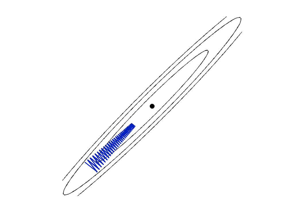
The figure below presents example functions and their minima. In the first illustration, there is a unique minimizer. In the second, there are an infinite number of minimizers, but all local minimizers are global minimizers. In the third example, there are many local minimizers that are not global minimizers.

Note that in our example, the two functions without suboptimal local minimizers share the property that for any two points w_1 and w_2, the line segment connecting (w_1,\Phi(w_1)) to (w_2,\Phi(w_2)) lies completely above the graph of the function. Such functions are called convex functions.
A function \Phi is convex if for all w_1, w_2 in \mathbb{R}^d and \alpha \in [0,1], \Phi(\alpha w_1 + (1-\alpha) w_2 )\leq \alpha\Phi(w_1)+(1-\alpha)\Phi(w_2)\,.
We will see shortly that convex functions are the class of functions where gradient descent is guaranteed to find an optimal solution.

Gradient descent
Suppose we want to minimize a differentiable function \Phi\colon\mathbb{R}^d \rightarrow \mathbb{R}. Most of the algorithms we will consider start at some point w_0 and then aim to find a new point w_1 with a lower function value. The simplest way to do so is to find a direction v such that \Phi is decreasing when moving along the direction v. This notion can be formalized by the following definition:
A vector v is a descent direction for \Phi at w_0 if \Phi(w_0 + tv) < \Phi(w_0) for some t>0.
For continuously differentiable functions, it’s easy to tell if v is a descent direction: if v^T \nabla \Phi(w_0) <0 then v is a descent direction.
To see this note that by Taylor’s theorem, \Phi(w_0 + \alpha v) = \Phi(w_0) + \alpha \nabla \Phi(w_0 + \tilde{\alpha} v)^T v for some \tilde{\alpha} \in [0,\alpha]. By continuity, if \alpha is small, we’ll have \nabla \Phi(w_0 + \tilde{\alpha} v)^Tv <0. Therefore \Phi(w_0 + \alpha v) < \Phi(w_0) and v is a descent direction.
This characterization of descent directions allows us to provide conditions as to when w minimizes \Phi.
The point w_\star is a local minimizer only if \nabla \Phi(w_\star) = 0\,.
Why is this true? Well, the point -\nabla \Phi(w_\star) is always a descent direction if it’s not zero. If w_\star is a local minimum, there can be no descent directions. Therefore, the gradient must vanish.
Gradient descent uses the fact that the negative gradient is always a descent direction to construct an algorithm: repeatedly compute the gradient and take a step in the opposite direction to minimize \Phi.
Gradient Descent
- Start from an initial point w_0 \in \mathbb{R}^d.
- At each step t=0,1,2,\dots:
- Choose a step size \alpha_t>0
- Set w_{t+1} = w_t - \alpha_t \nabla \Phi(w_t)
Gradient descent terminates whenever the gradient is so small that the iterates w_t no longer substantially change. Note now that there can be points where the gradient vanishes but where the function is not minimized. For example, maxima have this property. In general, points where the gradient vanishes are called stationary points. It is critically important to remember that not all stationary points are minimizers.

For convex \Phi, the situation is dramatically simpler. This is part of the reason why convexity is so appealing.
Let \Phi:\mathbb{R}^d\rightarrow \mathbb{R} be a differentiable convex function. Then w_\star is a global minimizer of \Phi if and only if \nabla \Phi(w_\star)=0.
To prove this, we need our definition of convexity: for any \alpha \in [0,1] and w\in\mathbb{R}^d, \Phi(w_\star + \alpha(w-w_\star)) = \Phi((1-\alpha)w_\star + \alpha w) \leq (1-\alpha) \Phi(w_\star) + \alpha \Phi(w) Here, the inequality is just our definition of convexity. Now, if we rearrange terms, we have \Phi(w) \geq \Phi(w_\star) + \frac{\Phi(w_\star + \alpha(w-w_\star)) - \Phi(w_\star)}{\alpha} Now apply Taylor’s theorem: there is now some \tilde{\alpha}\in[0,1] such that \Phi(w_\star + \alpha(w-w_\star)) - \Phi(w_\star)=\alpha \nabla \Phi(w_\star+ \tilde{\alpha}(w-w_\star))^T(w-w_\star). Taking the limit as \alpha goes to zero yields \Phi(w) \geq \Phi(w_\star) +\nabla \Phi(w_\star)^T(w-w_\star)\,.
But if \nabla \Phi(w_\star)=0, that means, \Phi(w) \geq \Phi(w_\star) for all w, and hence w_\star is a global minimizer.
Tangent hyperplanes always fall below the graphs of convex functions.
Let \Phi:\mathbb{R}^d\rightarrow \mathbb{R} be a differentiable convex function. Then for any u and v, we have \Phi(u) \geq \Phi(v) + \nabla \Phi(v)^T(u-v)\,.

A convex function cookbook
Testing if a function is convex can be tricky in more than two dimensions. But here are 5 rules that generate convex functions from simpler functions. In machine learning, almost all convex cost functions are built using these rules.
All norms are convex (this follows from the triangle inequality).
If \Phi is convex and \alpha \geq 0, then \alpha \Phi is convex.
If \Phi and \Psi are convex, then \Phi+\Psi is convex.
If \Phi and \Psi are convex, then h(w) = \max \{\Phi(w),\Psi(w)\} is convex.
If \Phi is convex and A is a matrix and b is a vector, then the function h(w)=\Phi(Aw+b) is convex.
All of these properties can be verified using only the definition of convex functions. For example, consider the 4th property. This is probably the trickiest of the list. Take two points w_1 and w_2 and \alpha \in [0,1]. Suppose, without loss of generality, that \Phi((1-\alpha)w_1+ \alpha w_2) \geq \Psi((1-\alpha) w_1 + \alpha w_2) \begin{aligned} h((1-\alpha) w_1 + \alpha w_2) &= \max \{\Phi((1- \alpha) w_1+ \alpha w_2),\Psi((1-\alpha) w_1 + \alpha w_2)\}\\ &= \Phi((1-\alpha) w_1+ \alpha w_2)\\ & \leq (1-\alpha) \Phi(w_1)+ \alpha \Phi(w_2)\\ &\leq (1-\alpha) \max\{\Phi(w_1),\Psi(w_1)\} + \alpha \max\{\Phi(w_2),\Psi(w_2)\}\\ & = (1-\alpha) h(w_1) + \alpha h(w_2) \end{aligned} Here, the first inequality follows because \Phi is convex. Everything else follows from the definition that h is the max of \Phi and \Psi. The reader should verify the other four assertions as an exercise. Another useful exercise is to verify that the SVM cost in the next section is convex by just using these five basic rules and the fact that the one dimensional function f(x)=mx+b is convex for any scalars m and b.
Applications to empirical risk minimization
For decision theory problems, we studied the zero-one loss that counts errors: \mathit{loss}(\hat{y},y) = \mathbb{1}\{ y\hat{y} < 0\} Unfortunately, this loss is not useful for the gradient method. The gradient is zero almost everywhere. As we discussed in the chapter on supervised learning, machine learning practice always turns to surrogate losses that are easier to optimize. Here we review three popular choices, all of which are convex loss functions. Each choice leads to a different important optimization problem that has been studied in its own right.
The support vector machine
Consider the canonical problem of support vector machine classification. We are provided pairs \left(x_{i},y_{i}\right), with x_{i}\in\mathbb{R}^{d} and y_{i}\in\left\{ -1,1\right\} for i=1,\ldots n (Note, the y labels are now in \{-1,1\} instead of \{0,1\}.) The goal is to find a vector w\in \mathbb{R}^d such that: \begin{aligned} w^{T}x_{i} & > 0\quad\text{ for }y_{i}=1\\ w^{T}x_{i} & < 0\quad\text{ for }y_{i}=-1 \end{aligned} Such a w defines a half-space where we believe all of the positive examples lie on one side and the negative examples on the other.
Rather than classifying these points exactly, we can allow some slack. We can pay a penalty of 1-y_i w^T x_i points that are not strongly classified. This motivates the hinge loss we encountered earlier and leads to the support vector machine objective: \text{minimize}_w\quad \sum_{i=1}^n \max\left\{1-y_i w^T x_i,0\right\} \,. Defining the function e(z) = \mathbb{1}\{ z\leq 1 \}, we can compute that the gradient of the SVM cost is -\sum_{i=1}^n e(y_i w^T x_i) y_i x_i \,. Hence, gradient descent for this ERM problem would follow the iteration w_{t+1} = w_t + \alpha \sum_{i=1}^n e(y_i w^T x_i) y_i x_i Although similar, note that this isn’t quite the perceptron method yet. The time to compute one gradient step is O(n) as we sum over all n inner products. We will soon turn to the stochastic gradient method that has constant iteration complexity and will subsume the perceptron algorithm.
Logistic regression
Logistic regression is equivalent to using the loss function \mathit{loss}(\hat y,y) = \log \left(1+\exp(-y\hat y)\right)\,. Note that even though this loss has a probabilistic interpretation, it can also just be seen as an approximation to the error-counting zero-one loss.
Least squares classification
Least squares classification uses the loss function \mathit{loss}(\hat y,y) = \tfrac{1}{2}(\hat y-y)^2\,. Though this might seem like an odd approximation to the error-counting loss, it leads to the maximum a posteriori (MAP) decision rule when minimizing the population risk. Recall the MAP rule selects the label that has highest probability conditional on the observed data.
It is helpful to keep the next picture in mind that summarizes how each of these different loss functions approximate the zero-one loss. We can ensure that the squared loss is an upper bound on the zero-one loss by dropping the factor 1/2.

Insights from quadratic functions
Quadratic functions are the prototypical example that motivate algorithms for differentiable optimization problems. Though not all insights from quadratic optimization transfer to more general functions, there are several key features of the dynamics of iterative algorithms on quadratics that are notable. Moreover, quadratics are a good test case for reasoning about optimization algorithms: if a method doesn’t work well on quadratics, it typically won’t work well on more complicated nonlinear optimization problems. Finally, note that ERM with linear functions and a squared loss is a quadratic optimization problem, so such problems are indeed relevant to machine learning practice.
The general quadratic optimization problem takes the form \Phi(w) = \tfrac{1}{2} w^T Q w - p^T w + r\,, where Q is a symmetric matrix, p is a vector, and r is a scalar. The scalar r only affects the value of the function, and plays no role in the dynamics of gradient descent. The gradient of this function is \nabla \Phi(w) = Qw - p\,. The stationary points of \Phi are the w where Qw = p. If Q is full rank, there is a unique stationary point.
The gradient descent algorithm for quadratics follows the iterations w_{t+1} = w_t - \alpha (Qw_t - p)\,. If we let w_\star be any stationary point of \Phi, we can rewrite this iteration as w_{t+1}-w_\star = (I-\alpha Q) (w_t - w_\star)\,. Unwinding the recursion yields the “closed form” formula for the gradient descent iterates w_{t}-w_\star = (I-\alpha Q)^t (w_0 - w_\star)\,.
This expression reveals several possible outcomes. Let \lambda_1 \geq \lambda_2 \geq \ldots \geq \lambda_d denote the eigenvalues of Q. These eigenvalues are real because Q is symmetric. First suppose that Q has a negative eigenvalue \lambda_d<0 and v is an eigenvector such that Qv = \lambda_d v. Then (I-\alpha Q)^t v = (1+\alpha |\lambda_d|)^t v which tends to infinity as t grows. This is because 1+\alpha |\lambda_d| is greater than 1 if \alpha>0. Hence, if \langle v, w_0-w_\star \rangle \neq 0, gradient descent diverges. For a random initial condition w_0, we’d expect this dot product will not equal zero, and hence gradient descent will almost surely not converge from a random initialization.
In the case that all of the eigenvalues of Q are positive, then choosing \alpha greater than zero and less than 1/\lambda_1 will ensure that 0\leq 1-\alpha \lambda_k <1 for all k. In this case, the gradient method converges exponentially quickly to the optimum w_\star: \begin{aligned} \Vert w_{t+1}-w_\star\Vert &= \Vert (I-\alpha Q) (w_t - w_\star)\Vert\\ &\leq \Vert I-\alpha Q\Vert \Vert w_t - w_\star \Vert \leq \left(1-\frac{\lambda_d}{\lambda_1}\right)\Vert w_t-w_\star\Vert\,. \end{aligned} When the eigenvalues of Q are all positive, the function \Phi is strongly convex. Strongly convex functions turn out to be the set of functions where gradient descent with a constant step size converges exponentially from any starting point.
Note that the ratio of \lambda_1 to \lambda_d governs how quickly all of the components converge to 0. Defining the condition number of Q to be \kappa = \lambda_1/\lambda_d and setting the step size \alpha = 1/\lambda_1, gives the bound \Vert w_{t}-w_\star\Vert \leq \left(1 - \kappa^{-1}\right)^t \Vert w_{0}-w_\star \Vert\,. This rate reflects what happens in practice: when there are small singular values, gradient descent tends to bounce around and oscillate as shown in the figure below. When the condition number of Q is small, gradient descent makes rapid progress towards the optimum.
There is one final case that’s worth considering. When all of the eigenvalues of Q are nonnegative but some of them are zero, the function \Phi is convex but not strongly convex. In this case, exponential convergence to a unique point cannot be guaranteed. In particular, there will be an infinite number of global minimizers of \Phi. If w_\star is a global minimizer and v is any vector with Qv=0, then w_\star+v is also a global minimizer. However, in the span of the eigenvectors corresponding to positive eigenvalues, gradient descent still converges exponentially. For general convex functions, it will be important to consider different parts of the parameter space to fully understand the dynamics of gradient methods.
Stochastic gradient descent
The stochastic gradient method is one of the most popular algorithms for contemporary data analysis and machine learning. It has a long history and has been “invented” several times by many different communities (under the names “least mean squares,” “backpropagation,” “online learning,” and the “randomized Kaczmarz method”). Most researchers attribute this algorithm to the initial work of Robbins and Monro from 1951 who solved a more general problem with the same method.Robbins and Monro, “A Stochastic Approximation Method,” The Annals of Mathematical Statistics, 1951, 400–407.
Consider again our main goal of minimizing the empirical risk with respect to a vector of parameters w, and consider the simple case of linear classification where w is d-dimensional and f(x_i;w) = w^Tx_i\,.
The idea behind the stochastic gradient method is that since the gradient of a sum is the sum of the gradients of the summands, each summand provides useful information about how to optimize the total sum. Stochastic gradient descent minimizes empirical risk by following the gradient of the risk evaluated on a single, random example.
Stochastic Gradient Descent
- Start from an initial point w_0 \in \mathbb{R}^d.
- At each step t=0,1,2,\dots:
- Choose a step size \alpha_t>0 and random index i \in [n].
- Set w_{t+1} = w_t - \alpha_t \nabla_{w_t} \mathit{loss}(f(x_i;w_t),y_i)
The intuition behind this method is that by following a descent direction in expectation, we should be able to get close to the optimal solution if we wait long enough. However, it’s not quite that simple. Note that even when the gradient of the sum is zero, the gradients of the individual summands may not be. The fact that w_\star is no longer a fixed point complicates the analysis of the method.
Example: revisiting the perceptron
Let’s apply the stochastic gradient method to the support vector machine cost loss. We initialize our half-space at some w_{0}. At iteration t, we choose a random data point (x_{i},y_{i}) and update w_{t+1}= w_{t}+\eta\begin{cases} y_{i}x_{i} &\text{if}~y_{i}w_{t}^{T}x_{i}\leq 1\\ 0 & \text{otherwise} \end{cases} As we promised earlier, we see that using stochastic gradient descent to minimize empirical risk with a hinge loss is completely equivalent to Rosenblatt’s Perceptron algorithm.
Example: computing a mean
Let’s now try to examine the simplest example possible. Consider applying the stochastic gradient method to the function \frac{1}{2n} \sum_{i=1}^n (w-y_i)^2\,, where y_1,\dots,y_n are fixed scalars. This setup corresponds to a rather simple classification problem where the x features are all equal to 1. Note that the gradient of one of the increments is \nabla \mathit{loss}(f(x_i;w),y) = w-y_i\,.
To simplify notation, let’s imagine that our random samples are coming to us in order \{1,2,3,4,...\} Start with w_1=0, use the step size \alpha_k = 1/k. We can then write out the first few equations: \begin{aligned} w_{2} & = w_{1}-w_{1}+y_{1}=y_{1}\\ w_{3} & = w_{2}-\frac{1}{2}\left(w_{2}-y_{2}\right)=\frac{1}{2}y_{1}+\frac{1}{2}y_{2}\\ w_{4} & = w_{3}-\frac{1}{3}\left(w_{3}-y_{3}\right) = \frac{1}{3}y_{1}+\frac{1}{3}y_{2}+\frac{1}{3}y_{3} \end{aligned} Generalizing from here, we can conclude by induction that w_{k+1} = \left(\frac{k-1}{k}\right)w_{k}+\frac{1}{k}y_{k}=\frac{1}{k}\sum_{i=1}^{k}y_{i}\,. After n steps, w_n is the mean of the y_i, and you can check by taking a gradient that this is indeed the minimizer of the ERM problem.
The 1/k step size was the originally proposed step size by Robbins and Monro. This simple example justifies why: we can think of the stochastic gradient method as computing a running average. Another motivation for the 1/k step size is that the steps tend to zero, but the path length is infinite.
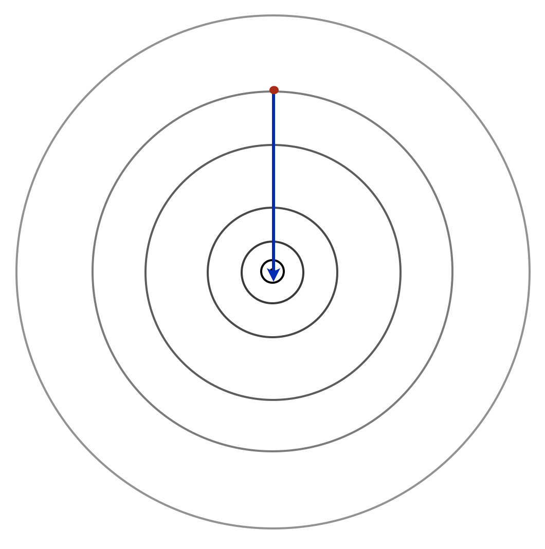
Moving to a more realistic random setting where the data might arrive in any order, consider what happens when we run the stochastic gradient method on the function R(w) = \tfrac{1}{2} \mathbb{E}[ (w-Y)^2]\,. Here Y is some random variable with mean \mu and variance \sigma^2. If we run for k steps with i.i.d. samples Y_i at each iteration, the calculation above reveals that w_k = \frac{1}{k} \sum_{i=1}^k Y_i\,. The associated cost is R(w_k) = \frac{1}{2} \mathop\mathbb{E}\left[ \left(\frac{1}{k} \sum_{i=1}^k Y_i-Y\right)^2\right] = \frac{1}{2k}\sigma^2 + \frac{1}{2}\sigma^2\,. Compare this to the minimum achievable risk R_\star. Expanding the definition R(w) = \tfrac{1}{2} \mathbb{E}[w^2 - 2 Y w + Y^2] = \tfrac{1}{2}w^2 - \mu w + \tfrac{1}{2}\sigma^2 + \tfrac{1}{2}\mu^2\,, we find that the minimizer is w_\star=\mu. Its cost is R_\star=R(w_\star) = \frac{1}{2} \sigma^2\,, and after n iterations, we have the expected optimality gap \mathop\mathbb{E}\left[R(w_n)-R_\star\right] = \frac{1}{2n}\sigma^2\,. This is the best we could have achieved using any estimator for w_\star given the collection of random draws. Interestingly, the incremental “one-at-a-time” method finds as good a solution as one that considers all of the data together. This basic example reveals a fundamental limitation of the stochastic gradient method: we can’t expect to generically get fast convergence rates without additional assumptions. Statistical fluctuations themselves prevent the optimality gap from decreasing exponentially quickly.
This simple example also helps give intuition on the convergence as we sample stochastic gradients. The figure below plots an example of each individual term in the summand, shaded with colors of blue to distinguish each term. The minimizing solution is marked with a red star. To the far left and far right of the figure, all of the summands will have gradients pointing in the same direction to the solution. However, as our iterate gets close to the optimum, we will be pointed in different directions depending on which gradient we sample. By reducing the step size, we will be more likely to stay close and eventually converge to the optimal solution.

Example: Stochastic minimization of a quadratic function
Let’s consider a more general version of stochastic gradient descent that follows the gradient plus some unbiased noise. We can model the algorithm as minimizing a function \Phi(w) where we follow a direction \nabla \Phi(w) + \nu where \nu is a random vector with mean zero and \mathop\mathbb{E}[\Vert \nu \Vert^2] = \sigma^2. Consider the special case where \Phi(w) is a quadratic function \Phi(w) = \tfrac{1}{2} w^T Q w - p^T w +r\,. Then the iterations take the form w_{t+1} = w_t - \alpha ( Qw_t -p + \nu_t)\,. Let’s consider what happens when Q is positive definite with maximum eigenvalue \lambda_1 and minimum eigenvalue \lambda_d >0. Then, if w_\star is a global minimizer of \Phi, we can again rewrite the iterations as w_{t+1}-w_\star = (I-\alpha Q) (w_t-w_\star) - \alpha\nu_t\,. Since we assume that the noise \nu_t is independent of all of the w_k with k \leq t, we have \mathop\mathbb{E}[ \Vert w_{t+1}-w_\star \Vert^2 ]\leq \Vert I-\alpha Q \Vert^2 \mathop\mathbb{E}[ \Vert w_t-w_\star\Vert^2 ] + \alpha^2\sigma^2\,. which looks like the formula we derived for quadratic functions, but now with an additional term from the noise. Assuming \alpha < 1/\lambda_1, we can unwind this recursion to find \mathop\mathbb{E}[ \Vert w_{t}-w_\star \Vert^2 ]\leq ( 1-\alpha \lambda_d)^{2t} \Vert w_0-w_\star\Vert^2 + \frac{\alpha \sigma^2}{\lambda_d}\,. From this expression, we see that gradient descent converges exponentially quickly to some ball around the optimal solution. The smaller we make \alpha, the closer we converge to the optimal solution, but the rate of convergence is also slower for smaller \alpha. This tradeoff motivates many of the step size selection rules in stochastic gradient descent. In particular, it is common to start with a large step size and then successively reduce the step size as the algorithm progresses.
Tricks of the trade
In this section, we describe key engineering techniques that are useful for tuning the performance of stochastic gradient descent. Every machine learning practitioner should know these simple tricks.
Shuffling. Even though we described the stochastic gradient method a sampling each gradient with replacement from the increments, in practice better results are achieved by simply randomly permuting the data points and then running SGD in this random order. This is called “shuffling,” and even a single shuffle can eliminate the pathological behavior we described in the example with highly correlated data. Recently, beginning with work by Gürbüzbalaban et al., researchers have shown that in theory, shuffling outperforms independent sampling of increments.Gürbüzbalaban, Ozdaglar, and Parrilo, “Why Random Reshuffling Beats Stochastic Gradient Descent,” Mathematical Programming, 2019, 1–36. The arguments for without-replacement sampling remain more complicated than the with-replacement derivations, but optimal sampling for SGD remains an active area of optimization research.
Step size selection. Step size selection in SGD remains a hotly debated topic. We saw above a decreasing stepsize 1/k solved our simple one dimensional ERM problem. However, a rule that works for an unreasonable number of cases is to simply pick the largest step size which does not result in divergence. This step will result in a model that is not necessarily optimal, but significantly better than initialization. By slowly reducing the step size from this initial large step size to successively smaller ones, we can zero in on the optimal solution.
Step decay. The step size is usually reduced after a fixed number of passes over the training data. A pass over the entire dataset is called an epoch. In an epoch, some number of iterations are run, and then a choice is made about whether to change the step size. A common strategy is to run with a constant step size for some fixed number of iterations T, and then reduce the step size by a constant factor \gamma. Thus, if our initial step size is \alpha, on the kth epoch, the step size is \alpha \gamma^{k-1}. This method is often more robust in practice than the diminishing step size rule. For this step size rule, a reasonable heuristic is to choose \gamma between 0.8 and 0.9. Sometimes people choose rules as aggressive as \gamma = 0.1.
Another possible schedule for the step size is called epoch doubling. In epoch doubling, we run for T steps with step size \alpha, then run 2T steps with step size \alpha/2, and then 4T steps with step size \alpha/4 and so on. Note that this provides a piecewise constant approximation to the function \alpha/k.
Minibatching. A common technique used to take advantage of parallelism is called minibatching. A minibatch is an average of many stochastic gradients. Suppose at each iteration we sample a \mathrm{batch}_k with m data points. The update rule then becomes w_{k+1} = w_{k} -\alpha_k \frac{1}{m}\sum_{j\in \mathrm{batch}_k} \nabla_w \mathit{loss}(f(x_j;w_k),y_j)\,. Minibatching reduces the variance of the stochastic gradient estimate of the true gradient, and hence tends to be a better descent direction. Of course, there are tradeoffs in total computation time versus the size of the minibatch, and these typically need to be handled on a case by case basis.
Momentum. Finally, we note that one can run stochastic gradient descent with momentum. Momentum mixes the current gradient direction with the previously taken step. The idea here is that if the previous weight update was good, we may want to continue moving along this direction. The algorithm iterates are defined as w_{k+1}=w_{k}-\alpha_{k}g_k\left(w_{k}\right) + \beta (w_{k}-w_{k-1})\,, where g_k denotes a stochastic gradient. In practice, these methods are very successful. Typical choices for \beta here are between 0.8 and 0.95. Momentum can provide significant accelerations, and should be considered an option in any implementation of SGM.
The SGD quick start guide
Newcomers to stochastic gradient descent often find all of these design choices daunting, and it’s useful to have simple rules of thumb to get going. We recommend the following:
- Pick as large a minibatch size as you can given your computer’s RAM.
- Set your momentum parameter to either 0 or 0.9. Your call!
- Find the largest constant stepsize such that SGD doesn’t diverge. This takes some trial and error, but you only need to be accurate to within a factor of 10 here.
- Run SGD with this constant stepsize until the empirical risk plateaus.
- Reduce the stepsize by a constant factor (say, 10)
- Repeat steps 4 and 5 until you converge.
While this approach may not be the most optimal in all cases, it’s a great starting point and is good enough for probably 90% of applications we’ve encountered.
Analysis of the stochastic gradient method
We now turn to a theoretical analysis of the general stochastic gradient method. Before we proceed, let’s set up some conventions. We will assume that we are trying to minimize a convex function R:\mathbb{R}^d \rightarrow \mathbb{R}. Let w_\star denote any optimal solution of R. We will assume we gain access at every iteration to a stochastic function g(w;\xi) such that \mathbb{E}_\xi[g(w; \xi)] = \nabla R(w)\,. Here \xi is a random variable which determines what our direction looks like. We additionally assume that these stochastic gradients are bounded so there exists a non-negative constants B such that \Vert g(w;\xi)\Vert \leq B\,.
We will study the stochastic gradient iteration w_{t+1}=w_{t}-\alpha_{t}g\left(w_{t};\xi_t\right)\,. Throughout, we will assume that the sequence \{\xi_j\} is selected i.i.d. from some fixed distribution.
We begin by expanding the distance to the optimal solution: \begin{aligned} \Vert w_{t+1} - w_\star \Vert^2 &= \Vert w_t - \alpha_t g_t(w_t;\xi_t) - w_\star \Vert^2 \\ &= \Vert w_t - w_\star\Vert^2 -2 \alpha_t \langle g_t( w_t;\xi_t), w_t- w_\star \rangle + \alpha_t^2 \Vert g_t(w_t; \xi_t) \Vert^2 \end{aligned}
We deal with each term in this expansion separately. First note that if we apply the law of iterated expectation \begin{aligned} \mathbb{E}[ \langle g_t(w_t;\xi_t), w_t - w_\star \rangle ] &= \mathbb{E}\left[\mathbb{E}_{\xi_t}[ \langle g_t(w_t;\xi_t), w_t - w_\star \rangle \mid \xi_0,\ldots,\xi_{t-1} ]\right]\\ &= \mathbb{E}\left[ \langle\mathbb{E}_{\xi_t}[ g_t(w_t;\xi_t) \mid \xi_0,\ldots,\xi_{t-1} ] , w_t - w_\star \rangle\right]\\ &= \mathbb{E}\left[ \langle \nabla R(w_t) , w_t - w_\star \rangle\right]\,. \end{aligned} Here, we are simply using the fact that \xi_t being independent of all of the preceding \xi_i implies that it is independent of w_t. This means that when we iterate the expectation, the stochastic gradient can be replaced by the gradient. The last term we can bound using our assumption that the gradients are bounded: \begin{aligned} \mathbb{E}[ \Vert g(w_t; \xi_t)\Vert^2] \leq B^2 \end{aligned}
Letting \delta_t := \mathbb{E}[\Vert w_{t}-w_\star\Vert^2], this gives \delta_{t+1} \leq \delta_t - 2 \alpha_t \mathbb{E}\left[ \langle \nabla R(w_t) , w_t - w_\star \rangle\right] + \alpha_t^2 B^2\,.
Now let \lambda_t = \sum_{j=0}^t \alpha_j denote the sum of all the step sizes up to iteration t. Also define the average of the iterates weighted by the step size \bar{w}_t = \lambda_t^{-1} \sum_{j=0}^t \alpha_j w_j\,. We are going to analyze the deviation of R(\bar{w}_t) from optimality.
Also let \rho_0 = \Vert w_0-w_\star\Vert. \rho_0 is the initial distance to an optimal solution. It is not necessarily a random variable.
To proceed, we just expand the following expression: \begin{aligned} \mathbb{E}\left[ R\left (\bar{w}_T \right) - R(w_\star) \right] & \leq \mathbb{E}\left[ \lambda_T^{-1} \sum_{t=0}^T \alpha_t( R(w_t) - R(w_\star) ) \right] \\ &\leq \lambda_T^{-1} \sum_{t=0}^T \alpha_t \mathbb{E}[ \langle \nabla R(x_t), w_t-w_\star \rangle ]\\ &\leq \lambda_T^{-1} \sum_{t=0}^T \tfrac{1}{2}(\delta_{t}-\delta_{t+1})+ \tfrac{1}{2} \alpha_t^2 B^2\\ & = \frac{\delta_0 - \delta_{T+1} + B^2 \sum_{t=0}^T \alpha_t^2}{2 \lambda_T}\\ & \leq \frac{\rho_0^2 + B^2 \sum_{t=0}^T \alpha_t^2}{2 \sum_{t=0}^T \alpha_t} \end{aligned} Here, the first inequality follows because R is convex (the line segments lie above the function, i.e., R(w_\star) \geq R(w_t) + \langle\nabla R(w_t), w_\star-w_t\rangle). The second inequality uses the fact that gradients define tangent planes to R and always lie below the graph of R, and the third inequality uses the recursion we derived above for \delta_t.
The analysis we saw gives the following result.Nemirovski et al., “Robust Stochastic Approximation Approach to Stochastic Programming,” SIAM Journal on Optimization 19, no. 4 (2009): 1574–1609.
Suppose we run the SGM on a convex function R with minimum value R_\star for T steps with step size \alpha. Define \alpha_{\mathrm{opt}} = \frac{\rho_0}{B\sqrt{T}}\qquad\text{and}\qquad \theta = \frac\alpha{\alpha_{\mathrm{opt}}}\,. Then, we have the bound \mathbb{E}[R(\bar{w}_T) - R_\star] \leq \left(\tfrac{1}{2} \theta + \tfrac{1}{2} \theta^{-1}\right) \frac{B \rho_0}{\sqrt{T}} \,.
This proposition asserts that we pay linearly for errors in selecting the optimal constant step size. If we guess a constant step size that is two-times or one-half of the optimal choice, then we need to run for at most twice as many iterations. The optimal step size is found by minimizing our upper bound on the suboptimality gap. Other step sizes could also be selected here, including diminishing step size. But the constant step size turns out to be optimal for this upper bound.
What are the consequences for risk minimization? First, for empirical risk, assume we are minimizing a convex loss function and searching for a linear predictor. Assume further that there exists a model with zero empirical risk. Let C be the maximum value of the gradient of the loss function, D be the largest norm of any example x_i and let \rho denote the minimum norm w such that R_S[w]=0. Then we have \mathbb{E}[R_S[\bar{w}_T]] \leq \frac{CD\rho}{\sqrt{T}} \,. we see that with appropriately chosen step size, the stochastic gradient method converges at a rate of 1/\sqrt{T}, the same rate of convergence observed when studying the one-dimensional mean computation problem. Again, the stochasticity forces us into a slow, 1/\sqrt{T} rate of convergence, but high dimensionality does not change this rate.
Second, if we only operate on samples exactly once, and we assume our data is i.i.d., we can think of the stochastic gradient method as minimizing the population risk instead of the empirical risk. With the same notation, we’ll have \mathbb{E}[R[\bar{w}_T]] -R_\star \leq \frac{CD\rho}{\sqrt{T}} \,. The analysis of stochastic gradient gives our second generalization bound of the book. What it shows is that by optimizing over a fixed set of T data points, we can get a solution that will have low cost on new data. We will return to this observation in the next chapter.
Implicit convexity
We have thus far focused on convex optimization problems, showing that gradient descent can find global minima with modest computational means. What about nonconvex problems? Nonconvex optimization is such a general class of problems that in general it is hard to make useful guarantees. However, ERM is a special optimization problem, and its structure enables nonconvexity to enter in a graceful way.
As it turns out there’s a “hidden convexity” of ERM problems which shows that the predictions should converge to a global optimum even if we can’t analyze to where exactly the model converges. We will show this insight has useful benefits when models are overparameterized or nonconvex.
Suppose we have a loss function \mathit{loss} that is equal to zero when \hat{y} = y and is nonnegative otherwise. Suppose we have a generally parameterized function class \{ f(x;w) \colon w\in\mathbb{R}^d\} and we aim to find parameters w that minimize the empirical risk. The empirical risk R_S[w] =\frac{1}{n} \sum_{i=1}^n \mathit{loss}(f(x_i;w),y_i) is bounded below by 0. Hence if we can find a solution with f(x_i;w)=y_i for all i, we would have a global minimum not a local minimum. This is a trivial observation, but one that helps focus our study. If during optimization all predictions f(x_i;w) converge to y_i for all i, we will have computed a global minimizer. For the sake of simplicity, we specialize to the square loss in this section: \mathit{loss}(f(x_i;w),y_i) = \tfrac{1}{2} (f(x_i;w)-y_i)^2 The argument we develop here is inspired by the work of Du et al. who use a similar approach to rigorously analyze the convergence of two layer neural networks.Du et al., “Gradient Descent Provably Optimizes over-Parameterized Neural Networks,” in International Conference on Learning Representations, 2019. Similar calculations can be made for other losses with some modifications of the argument.
Convergence of overparameterized linear models
Let’s first consider the case of linear prediction functions f(x;w) = w^T x\,. Define y = \begin{bmatrix} y_1\\ \vdots \\ y_n \end{bmatrix}\qquad \qquad \text{and}\qquad \qquad X = \begin{bmatrix} x_1^T \\ \vdots \\x_n^T \end{bmatrix}\,. We can then write the empirical risk objective as R_S[w]=\frac1{2n}\|Xw-y\|^2\,. The gradient descent update rule has the form w_{t+1} = w_t - \alpha X^T (X w_t-y)\,. We pull the scaling factor 1/n into the step size for notational convenience. Now define the vector of predictions \hat{y}_t = \begin{bmatrix} f(x_1;w_t) \\ \vdots \\ f(x_n;w_t) \end{bmatrix}\,. For the linear case, the predictions are given by \hat{y}_k = X w_k. We can use this definition to track the evolution of the predictions instead of the parameters w. The predictions evolve according to the rule \hat{y}_{t+1} = \hat{y}_t - \alpha X X^T (\hat{y}_t-y)\,. This looks a lot like the gradient descent algorithm applied to a strongly convex quadratic function that we studied earlier. Subtracting y from both sides and rearranging shows \hat{y}_{t+1}-y = (I - \alpha X X^T) (\hat{y}_t-y)\,. This expression proves that as long as XX^T is strictly positive definite and \alpha is small enough, then the predictions converge to the training labels. Keep in mind that X is n\times d and a model is overparameterized if d>n. The n\times n matrix XX^T has a chance of being strictly positive definite in this case.
When we use a sufficiently small and constant step size \alpha, our predictions converge at an exponential rate. This is in contrast to the behavior we saw for gradient methods on overdetermined problems. Our general analysis of the weights showed that the convergence rate might be only inverse polynomial in the iteration counter. In the overparameterized regime, we can guarantee the predictions converge more rapidly than the weights themselves.
The rate in this case is governed by properties of the matrix X. As we have discussed we need the eigenvalues of XX^T to be positive, and we’d ideally like that the eigenvalues are all of similar magnitude.
First note that a necessary condition is that d, the dimension, must be larger than n, the number of data points. That is, we need to have an overparameterized model in order to ensure exponentially fast convergence of the predictions. We have already seen that such overparameterized models make it possible to interpolate any set of labels and to always force the data to be linearly separable. Here, we see further that overparameterization encourages optimization methods to converge in fewer iterations by improving the condition number of the data matrix.
Overparameterization can also help accelerate convergence. Recall that the eigenvalues of XX^T are the squares of the singular values of X. Let us write out a singular value decomposition X = USV^T\,, where S is a diagonal matrix of singular values (\sigma_1,\ldots, \sigma_n). In order to improve the condition number of this matrix, it suffices to add a feature that is concentrated in the span of the singular vectors with small singular values. How to find such features is not always apparent, but does give us a starting point as to where to look for new, informative features.
Convergence of nonconvex models
Surprisingly, this analysis naturally extends to nonconvex models. With some abuse of notation, let \hat y = f(x;w)\in\mathbb{R}^n denote the n predictions of some nonlinear model parameterized by the weights w on input x. Our goal is to minimize the squared loss objective \frac12\|f(x;w)-y\|^2\,. Since the model is nonlinear this objective is no longer convex. Nonetheless we can mimic the analysis we did previously for overparameterized linear models.
Running gradient descent on the weights gives w_{t+1} = w_t - \alpha \mathsf{D}f (x;w_t)(\hat{y}_t - y)\,, where \hat y_t=f(x;w_t) and \mathsf{D}f is the Jacobian of the predictions with respect to w. That is, \mathsf{D}f (x;w) is the d\times n matrix of first order derivatives of the function f(x;w) with respect to w. We can similarly define the Hessian operator H(w) to be the n \times d \times d array of second derivatives of f(x;w). We can think of H(w) as a quadratic form that maps pairs of vectors (u,v) \in \mathbb{R}^{d\times d} to \mathbb{R}^n. With these higher order derivatives, Taylor’s theorem asserts \begin{aligned} \hat{y}_{t+1} &= f(x,w_{t+1})\\ &= f(x,w_t) + \mathsf{D}f (x;w_t)^T(w_{t+1}-w_t) \\ &\qquad\qquad+ \int_0^1 H(w_t+s (w_{t+1}-w_t)) (w_{t+1}-w_t, w_{t+1}-w_t) \mathrm{d}s\,. \end{aligned} Since w_t are the iterates of gradient descent, this means that we can write the prediction as \begin{aligned} \hat{y}_{t+1} &= \hat{y}_t -\alpha \mathsf{D}f(x;w_t)^T \mathsf{D}f(x;w_t)(\hat{y_t} - y) + \alpha \epsilon_t \,, \end{aligned} where \epsilon_t = \alpha \int_0^1 H(w_t+s (w_{t+1}-w_t)) \left( \mathsf{D}f(x;w_t) (\hat{y}_t - y),\mathsf{D}f(x;w_t) (\hat{y}_t - y)\right)\mathrm{d}s\,. Subtracting the labels y from both sides and rearranging terms gives the recursion \hat{y}_{t+1}-y = (I - \alpha \mathsf{D}f(x;w_t)^T \mathsf{D}f(x;w_t))(\hat{y}_t - y) + \alpha \epsilon_t\,. If \epsilon_t vanishes, this shows that the predictions again converge to the training labels as long as the eigenvalues of \mathsf{D}f(x;w_t)^T \mathsf{D}f(x;w_t) are strictly positive. When the error vector \epsilon_t is sufficiently small, similar dynamics will occur. We expect \epsilon_t to not be too large because it is quadratic in the distance of y_t to y and because it is multiplied by the step size \alpha which can be chosen to be small.
The nonconvexity isn’t particularly disruptive here. We just need to make sure our Jacobians have full rank most of the time and that our steps aren’t too large. Again, if the number of parameters are larger than the number of data points, then these Jacobians are likely to be positive definite as long as we’ve engineered them well. But how exactly can we guarantee that our Jacobians are well behaved? We can derive some reasonable ground rules by unpacking how we compute gradients of compositions of functions. More on this follows in our chapter on deep learning.
Regularization
The topic of regularization belongs somewhere between optimization and generalization and it’s one way of connecting the two. Hence, we will encounter it in both chapters. Indeed, one complication with optimization in the overparameterized regime is that there is an infinite collection of models that achieve zero empirical risk. How do we break ties between these and which set of weights should we prefer?
To answer this question we need to take a step back and remember that the goal of supervised learning is not just to achieve zero training error. We also care about performance on data outside the training set, and having zero loss on its own doesn’t tell us anything about data outside the training set.
As a toy example, imagine we have two sets of data X_{\mathrm{train}} and X_{\mathrm{test}} where X_{\mathrm{train}} has shape n \times d and X_{\mathrm{test}} is m \times d. Let y_{\mathrm{train}} be the training labels and let q be an m-dimensional vector of random labels. Then if d>(m+n) we can find weights w such that \begin{bmatrix} X_{\mathrm{train}} \\ X_{\mathrm{test}} \end{bmatrix} w = \begin{bmatrix} y_{\mathrm{train}} \\ q \end{bmatrix}\,. That is, these weights would produce zero error on the training set, but error no better than random guessing on the testing set. That’s not desired behavior! Of course this example is pathological, because in reality we would have no reason to fit random labels against the test set when we create our model.
The main challenge in supervised learning is to design models that achieve low training error while performing well on new data. The main tool used in such problems is called regularization. Regularization is the general term for taking a problem with infinitely many solutions and biasing its solution towards a smaller subset of solution space. This is a highly encompassing notion.
Sometimes regularization is explicit insofar as we have a desired property of the solution in mind which we exercise as a constraint on our optimization problem. Sometimes regularization is implicit insofar as algorithm design choices lead to a unique solution, although the properties of this solution might not be immediately apparent.
Here, we take an unconventional tack of working from implicit to explicit, starting with stochastic gradient descent.
Implicit regularization by optimization
Consider again the linear case of gradient descent or stochastic gradient descent w_{t+1} = w_t - \alpha e_t x_t\,, where e_t is the gradient of the loss at the current prediction. Note that if we initialize w_0=0, then w_t is always in the span of the data. This can be seen by simple induction. This already shows that even though general weights lie in a high dimensional, SGD searches over a space with dimension at most n, the number of data points.
Now suppose we have a nonnegative loss with \frac{\partial \mathit{loss}(z,y)}{\partial z} = 0 if and only if y=z. This condition is satisfied by the square loss, but not hinge and logistic losses. For such losses, at optimality we have for some vector v that:
- Xw = y\,, because we have zero loss.
- w = X^T v\,, because we are in the span of the data.
Under the mild assumption that our examples are linearly independent, we can combine these equations to find that w=X^T(XX^T)^{-1}y\,. That is, when we run stochastic gradient descent we converge to a very specific solution. Even though we were searching through an n-dimensional space, we converge to a unique point in this space.
This special w is the minimum Euclidean norm solution of Xw=y. In other words, out of all the linear prediction functions that interpolate the training data, SGD selects the solution with the minimal Euclidean norm. To see why this solution has minimal norm, suppose that \hat{w} = X^T\alpha + v with v orthogonal to all x_i. Then we have X\hat{w} = XX^T\alpha + Xv = XX^T\alpha \,. Which means \alpha is completely determined and hence \hat{w} = X^T(XX^T)^{-1}y+ v. But now \Vert \hat{w}\Vert^2 = \Vert X^T(XX^T)^{-1}y\Vert^2 + \Vert v \Vert^2\,. Minimizing the right hand side shows that v must equal zero.
We now turn to showing that such minimum norm solutions have important robustness properties that suggest that they will perform well on new data. In the next chapter, we will prove that these methods are guaranteed to perform well on new data under reasonable assumptions.
Margin and stability
Consider a linear predictor that makes no classification errors and hence perfectly separates the data. Recall that the decision boundary of this predictor is the hyperplane \mathcal{B}= \{z\,:\,w^Tz = 0\} and the margin of the predictor is the distance of the decision boundary from to data: \mathrm{margin}(w) = \min_i \operatorname{dist}\left(x_i,\mathcal{B}\right)\,. Since we’re assuming that w correctly classifies all of the training data, we can write the margin in the convenient form \operatorname{margin}(w) = \min_i \frac{y_i w^Tx_i}{\Vert w\Vert}\,.
Ideally, we’d like our data to be far away from the boundary and hence we would like our predictor to have large margin. The reasoning behind this desideratum is as follows: If we expect new data to be similar to the training data and the decision boundary is far away from the training data, then it would be unlikely for a new data point to lie on the wrong side of the decision boundary. Note that margin tells us how large a perturbation in the x_i can be handled before a data point is misclassified. It is a robustness measure that tells us how sensitive a predictor is to changes in the data itself.
Let’s now specialize margin to the interpolation regime described in the previous section. Under the assumption that we interpolate the labels so that w^Tx_i=y_i, we have \operatorname{margin}(w) = \Vert w\Vert^{-1}\,. If we want to simultaneously maximize margin and interpolate the data, then the optimal solution is to choose the minimum norm solution of Xw=y. This is precisely the solution found by SGD and gradient descent.
Note that we could have directly tried to maximize margin by solving the constrained optimization problem \begin{array}{ll} \text{minimize} & \Vert w \Vert^2\\ \text{subject to} & y_i w^Tx_i \geq 1\,. \end{array} This optimization problem is the classic formulation of the support vector machine. The support vector machine is an example of explicit regularization. Here we declare exactly which solution we’d like to choose given that our training error is zero. Explicit regularization of high dimensional models is as old as machine learning. In contemporary machine learning, however, we often have to squint to see how our algorithmic decisions are regularizing. The tradeoff is that we can run faster algorithms with implicit regularizers. But it’s likely that revisiting classic regularization ideas in the context of contemporary models will lead to many new insights.
The representer theorem and kernel methods
As we have discussed so far, it is common in linear methods to restrict the search space to the span of the data. Even when d is large (or even infinite), this reduces the search problem to one in an n-dimensional space. It turns out that under broad generality, solutions in the span of the data are optimal for most optimization problems in prediction. Here, we make formal an argument we first introduced in our discussion of features: for most empirical risk minimization problems, the optimal model will lie in the span of the training data.
Consider the penalized ERM problem \text{minimize} \frac{1}{n} \sum_{i=1}^n \mathit{loss}(w^T x_i, y_i) + \lambda \Vert w\Vert^2 Here \lambda is called a regularization parameter. When \lambda=0, there are an infinite number of w that minimize the ERM problem. But for any \lambda>0, there is a unique minimizer. The term regularization refers to adding some prior information to an optimization problem to make the optimal solution unique. In this case, the prior information is explicitly encoding that we should prefer w with smaller norms if possible. As we discussed in our chapter on features, smaller norms tend to correspond to simpler solutions in many feature spaces. Moreover, we just described that minimum norm solutions themselves could be of interest in machine learning. A regularization parameter allows us to explicitly tune the norm of the optimal solution.
For our penalized ERM problem, using the same argument as above, we can write any w as w = X^T \beta + v for some vectors \beta and v with v^Tx_i=0 for all i. Plugging this equation into the penalized ERM problem yields \text{minimize}_{\beta,v} \frac{1}{n} \sum_{i=1}^n \mathit{loss}(\beta^T X x_i,y_i) + \lambda \Vert X^T \beta \Vert^2 + \lambda \Vert v\Vert^2\,. Now we can minimize with respect to v, seeing that the only option is to set v=0. Hence, we must have that the optimum model lies in the span of the data: w = X^T \beta This derivation is commonly called the representer theorem in machine learning. As long as the cost function only depends on function evaluations f(x_i)=w^Tx_i and the cost increases as a function of \Vert w\Vert, then the empirical risk minimizer will lie in the span of the data.
Define the kernel matrix of the training data K = XX^T. We can then rewrite the penalized ERM problem as \text{minimize}_{\beta} \frac{1}{n} \sum_{i=1}^n \mathit{loss}(e_i^T K\beta,y_i) + \lambda \beta^T K \beta\,, where e_i is the standard Euclidean basis vector. Hence, we can solve the machine learning problem only using the values in the matrix K, searching only for the coefficients \beta in the kernel expansion.
The representer theorem (also known as the kernel trick) tells us that most machine learning problems reduce to a search in n dimensional space, even if the feature space has much higher dimension. Moreover, the optimization problems only care about the values of dot products between data points. This motivates the use of the kernel functions described in our discussion of representation: kernel functions allow us to evaluate dot products of vectors in high dimensional spaces often without ever materializing the vectors, reducing high-dimensional function spaces to the estimation of weightings of individual data points in the training sample.
Squared loss methods and other optimization tools
This chapter focused on gradient methods for minimizing empirical risk, as these are the most common methods in contemporary machine learning. However, there are a variety of other optimization methods that may be useful depending on the computational resources available and the particular application in question.
There are a variety of optimization methods that have proven fruitful in machine learning, most notably constrained quadratic programming for solving support vector machines and related problems. In this section we highlight least squares methods which are attractive as they can be solved by solving linear systems. For many problems, linear systems solves are faster than iterative gradient methods, and the computed solution is exact up to numerical precision, rather than being approximate.
Consider the optimization problem \begin{array}{ll} \text{minimize}_w & \tfrac{1}{2}\sum_{i=1}^n (y_i-w^T x_i)^2 \,. \end{array} The gradient of this loss function with respect to w is given by -\sum_{i=1}^n (y_i-w^T x_i)x_i \,. If we let y denote the vector of y labels and X denote the n\times d matrix X = \begin{bmatrix} x_1^T\\ x_2^T \\ \vdots \\ x_n^T \end{bmatrix}\,, then setting the gradient of the least squares cost equal to zero yields the solution w = (X^T X)^{-1} X^T y\,. For many problems, it is faster to compute this closed form solution than it is to run the number of iterations of gradient descent required to find a w with small empirical risk.
Regularized least squares also has a convenient closed form solution. The penalized ERM problem where we use a square loss is called the ridge regression problem: \begin{array}{ll} \text{minimize}_w & \tfrac{1}{2}\sum_{i=1}^n (y_i-w^T x_i)^2 +\lambda \Vert w\Vert^2 \end{array} Ridge regression can be solved in the same manner as above, yielding the optimal solution w = (X^T X+ \lambda I)^{-1} X^T y\,. There are a few other important problems solvable by least squares. First, we have the identity (X^T X+ \lambda I_d)^{-1} X^T = X^T (X X^T+ \lambda I_n)^{-1}\,. this means that we can solve ridge regression either by solving a system in d equations and d unknowns or n equations and n unknowns. In the overparameterized regime, we’d choose the formulation with n parameters. Moreover, as we described above, the minimum norm interpolating problem \begin{array}{ll} \text{minimize} & \Vert w \Vert^2\\ \text{subject to} & w^Tx_i = y_i\,. \end{array} is solved by w= X (X X^T)^{-1}y. This shows that the limit as \lambda goes to zero in ridge regression is this minimum norm solution.
Finally, we note that for kernelized problems, we can simply replace the matrix X X^T with the appropriate kernel K. Hence, least squares formulations are extensible to solve prediction problems in arbitrary kernel spaces.
Chapter notes
Mathematical optimization is a vast field, and we clearly are only addressing a very small piece of the puzzle. For an expanded coverage of the material in this chapter with more mathematical rigor and implementation ideas, we invite the reader to consult the recent book by Wright and Recht.Wright and Recht, Optimization for Data Analysis (Cambridge University Press, 2021).
The chapter focuses mostly on iterative, stochastic gradient methods. Initially invented by Robbins and Monro for solving systems of equations in random variables,Robbins and Monro, “A Stochastic Approximation Method.” stochastic gradient methods have played a key role in pattern recognition since the Perceptron. Indeed, it was very shortly after Rosenblatt’s invention that researchers realized the Perceptron was solving a stochastic approximation problem. Of course, the standard perceptron step size schedule does not converge to a global optimum when the data is not separable, and this lead to a variety of methods to fix the problem. Many researchers employed the Widrow-Hoff “Least-Mean-Squares” rule which in modern terms is minimizing the empirical risk associated with a square loss by stochastic gradient descent.Widrow and Hoff, “Adaptive Switching Circuits,” in Institute of Radio Engineers, Western Electronic Show and Convention, Convention Record, 1960, 96–104. Aizerman and his colleagues determined not only how to apply stochastic gradient descent to linear functions, but how to operate in kernel spaces as well.Aizerman, Braverman, and Rozonoer, “The Robbins-Monro Process and the Method of Potential Functions,” Automation and Remote Control 26 (1965): 1882–85. Of course, all of these methods were closely related to each other, but it took some time to put them all on a unified footing. It wasn’t until the 1980s with a full understanding of complexity theory, that optimal step sizes were discovered for stochastic gradient methods by Nemirovski and Yudin.Nemirovski and Yudin, Problem Complexity and Method Efficiency in Optimization (Wiley, 1983). More surprisingly, it was not until 2007 that the first non-asymptotic analysis of the perceptron algorithm was published.Shalev-Shwartz, Singer, and Srebro, “Pegasos: Primal Estimated Sub-GrAdient SOlver for SVM,” in International Conference on Machine Learning, 2007.
Interestingly, it wasn’t again until the early 2000s that stochastic gradient descent became the default optimization method for machine learning. There tended to be a repeated cycle of popularity for the various optimization methods. Global optimization methods like linear programming were determined effective in the 1960s for pattern recognition problems,Mangasarian, “Linear and Nonlinear Separation of Patterns by Linear Programming,” Operations Research 13, no. 3 (1965): 444–52. supplanting interest in stochastic descent methods. Stochastic gradient descent was rebranded as back propagation in the 1980s, but again more global methods eventually took center stage. Mangasarian, who was involved in both of these cycles, told us in private correspondence that linear programming methods were always more effective in terms of their speed of computation and quality of solution.
Indeed this pattern was also followed in optimization. Nemirovski and Nesterov did pioneering work in iterative gradient and stochastic gradient methods . But they soon turned to developing the foundations of interior point methods for solving global optimization problems.Nesterov and Nemirovskii, Interior-Point Polynomial Methods in Convex Programming (SIAM, 1994). In the 2000s, they republished their work on iterative methods, leading to a revolution in machine learning.
It’s interesting to track this history and forgetting in machine learning. Though these tools are not new, they are often forgotten and replaced. It’s perhaps time to revisit the non-iterative methods in light of this.